Due Monday May 15, 2000 (or up to May 22 with late penalty)
In this assignment you will use some of the techniques you've learned to do some basic bitmap operations. Very frequently when processing images, it is useful to know the set of connected components in the image. "Circle of radius 20 centered at (212,113)" is more useful than the raw pixels when you're trying to figure out what's in the image.
For our purposes, we will always deal in monochrome images, where each pixel is either black or white (black is the background). One way to arrange this is to threshold the input image. For example, typically the input pixels are defined as RGB (red, green, blue) triplets, where each color ranges from 0 to 255. We can define a threshold function based on the sum of the three colors. If the total is greater than 3 * (255/2), we make the pixel a 1 (representing white), otherwise we make it 0 (for black). (A 1 isn't actually white in our case, but all we care about is that there are exactly two possible values.)
The pixel data is just a one byte color index. To get the actual RGB values, we need to use this number to access the palette, a table of color values. For example, a pixel with value "73" means that the pixel's color is defined by entry 73 in the palette. Each palette entry is a structure containing R, G, and B values. The skeleton code creates a palette[ ] array which you can access.
So, to start with, we have an image (essentially a two-dimensional array of pixels) where each pixel has the value 0 or 1. The images will be 8-bit (256-color), so each pixel is a one-byte value.
First, we need to define the concept of neighbors of a pixel. There are two ways to define this. The 4-neighborhood of a pixel are the four pixels to the north, south, east, and west. The 8-neighborhood also includes the diagonals.
Figure 1: the 4-neighbors and 8-neighbors of a pixel.
We define a connected component of an image to be a set of pixels that are connected by a chain of neighbors. Thus, a vertical or horizontal line of pixels would be connected under either definition, but a 45-degree diagonal line that is only one pixel wide would only be connected under the 8-neighborhood definition. The pixels in a connected component can be thought of as an equivalence class.
There is a very simple algorithm to scan an image and construct the connected components, using the disjoint set ADT. In principle, it is:
for each pixel p in image  // i.e. each non-zero pixel

    for each neighbor n  // i.e. each non-zero neighbor

        union the equivalence classes of the
two pixels
A number of changes need to be made in order to have a practical algorithm, however.
We will use 256x256 images, or 65536 pixels. The book's algorithm tells us to start with a forest of 64K individual trees, and then union them as we discover adjacencies. This forest would be bigger than the image itself! Instead of assigning each pixel its own equivalence class to start, we will only create a new class when we find a new pixel that can't be merged with any neighbors.
The equivalence classes will be stored in a 256-element array (of ints). Let's call this array DJ. Each pixel in the image will be modified to hold an index into this array. Thus, we can determine the class of a pixel by following these indexes in the DJ array until we find a root class. The modified algorithm becomes:
for each pixel p in image

    temporarily assign p to a new equivalence class, by itself

    // i.e., set the value of pixel p to some unused number, and
set that entry in DJ

    if p has neighbors, then for each neighbor n

        set p's class to the union of p's
current class and n's class

        // you will need to do find
operations in the previous step

    else, if p has no neighbors,

        let p end in a new equivalence class
You'll want to use an integer variable to keep track of the next free class number (start with 1, not 0). The pixels in our images are only one byte, so we can't handle classes numbered higher than 255. If you allocate a new number for every white pixel you see, you will quickly run out of classes. So, you should only use a new class number when the pixel has no neighbors.
Since not all pixels will have a defined equivalence class until the algorithm finishes, how can we examine the neighbors in the code above? The answer is that you only need to look at the neighbors you've already processed. Assuming we are scanning left-to-right, top-to-bottom:
Only pixels 1-4 need to be checked. If any of those pixels are non-zero, we union the current pixel with each of them in turn. No new class needs to be used. Neighbors 5-8 will be scanned later, and at that time they will be union'ed with the current pixel if necessary. Of course if we are using 4-neighborhoods, then only pixels 2 and 4 need to be checked. Complete pseudocode:
for each pixel p in image

    temporarily assign p to a new equivalence class, by itself

    // i.e., set the value of pixel p to some unused number, and
set that entry in DJ

    if p has neighbors (1-4, or 2 and 4), then for each neighbor
n

        set p's class to the union of p's
current class and n's class

        // you will need to do find
operations in the previous step

    else, if p has no neighbors,

        let p end in a new equivalence class
An example will be helpful. Suppose we are scanning the following image using 4-neighborhoods:
When we reach the end of the first line, we hit our first white pixel. It has no neighbors above or to the left, so we assign it a new class numbered 1. We also update the disjoint set array so that element 1 is marked as being a root.
At the beginning of the second line, we find another new pixel that needs to be given a new equivalence class (2).
The next pixel does have a neighbor to its left. We can temporarily assign this pixel to equivalence class 3 (or zero). We use the Find operation to figure out what class our west neighbor belongs to (the class is 2). We then use the Union operation to merge the two classes together. The pixel is assigned to whatever the Union function returns.
Note that in order to conserve class numbers, the Union function should not return the temporary class value. One way to do this is to always use zero as the temporary class, and code Union so that if it sees a zero class, that one is always made a child of the other. We don't care about the temporary class, because we're going to immediately throw out that value when we assign the pixel to what Union returns.
Finally, we get to the 4th white pixel. It has two neighbors. So, first we assign the pixel to a temporary class, e.g. 0. We then Union with the north neighbor, which returns 1 as the merged class, so the pixel now contains 1. Then we Union with the left neighbor. The result will either be 1 or 2, and we assign that as the final pixel value.
A longer example, again using 4-neighborhoods. To the right, the state of the disjoint set structure (the DJ array) is shown after processing each row of the image, assuming union-by-size (see next section). The gray cells represent unused class names.
Rows 1,2: The first two lines are like the first example. The second 1 is bold to indicate that two classes (1 and 2) were union'ed, and 1 was chosen as the winner.
Row 3: The next pixel has no neighbors to the north or west, so it gets a new class of 3. The next pixel has to be union'ed twice. First, the north neighbor is checked. Although it has a value of 2, when we do a Find we discover that the root is 1, so we assign the pixel a value of 1. Then we union with the left neighbor (3). Assuming the 1 wins again, the class 3 will be merged with class 1.
Row 4: The last line is similar, introducing a class 4 and then merging it with class 1 (since Find(3) returns 1).
I recommend that you use union-by-size to speed up your code. This means that, in the DJ array, roots should contain a negative value corresponding to the size of that class. When you create a new class for a pixel, set the root to -1. When you union two classes, make the smaller (i.e. less negative) class a child of the larger (more negative). The larger root will be the sum of the two old sizes. The smaller root will now point to the larger one. This is exactly like what we talked about in class and what's shown in the book.
If for some reason you have trouble getting this to work, it is not required. You can compute the counts for each class in a separate pass at the end when you print out the results discussed below.
After you scan the entire image, do a second scan and update each pixel to its class value. That is, set pixel = Find(pixel). This will cause all equivalent pixels to have the same value (which will be 1-255, since the DJ array is only 256 elements large).
For each class, compute the count of pixels in the class. Also compute the center of the class. This is easily done by adding up the row and column values for each pixel in the class, and dividing by the count.
Use any sorting algorithm you like (I used Insertion Sort) to sort the classes by size. Your program should print out the following information:
Summary: your program must do the following:
Turn in hardcopy and online. Comment your code! Commenting will be worth 10% of your grade. If you are getting stuck, skip the sorting and skip handling 8-neighborhoods. Concentrate on getting the core code done first. Your hardcopy must include the printed output of your program--not the images, but the sorted class information. Indicate for each run which file was the input and whether you were using 4- or 8-neighborhoods.
This assignment is a bit harder than the Split homework was, although you don't have to write much recursive code this time. The following source and input files are provided.
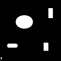
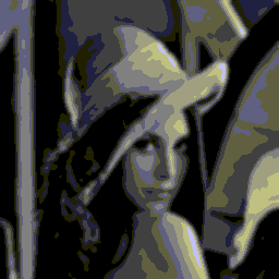
The sample solution expects to read the input file from standard in, and always writes output to "out.bmp". Input files must be 256x256 8-bit Windows BMP files. The I/O code provided is not that robust and will have trouble with other bitmap files.
About bitmap files: an 8-bit bitmap file can hold up 256 colors. However, instead of storing the color values directly, an indirect color value is stored in each pixel. The beginning of the file contains a palette, which is a table of 256 actual color values. These values are specified as RGB triplets, using 3 bytes each (plus one padding byte). The value stored in a pixel, e.g. 12, is used as an index into the palette. Thus, a pixel value of 12 could mean any color, depending on what the palette contains. For our purposes, this means that you can store any value from 0 to 255 into the pixels and get a distinct color (although many are similar).
Run the program using the following command lines. The second tells the
program to use 8-neighborhoods instead of 4-neighborhoods.
hw5 < input.bmp
hw5 8 < input.bmp
Windows bitmaps are stored from the bottom up. What you think is row 0 is actually the bottom row of the image. This doesn't matter for the algorithm, but you need to correct when you print out the coordinate information for each class. Simply print '(255-row)' instead of just 'row'. You don't need to make any correction for the column data.
You should abort your program if you use up all 255 available classes. You should check for this case because you may get confusing error behavior if you run off the end of the DJ array without realizing it. It's very easy to run out if you create a medium complexity image, especially if you are using 4-neighborhood.
The skeleton program provides two functions, readbmp and writebmp. Readbmp loads in the header information from the file and spits an exact copy to the output. It also loads the palette (which you don't need to mess with) and the pixel data into arrays. You modify the pixel data in place, and call writebmp when you are done. If you have assigned each component a different value, it will appear in a different color in the output file.
The sample solution prints some extra information about colors--you don't have to do this.
 Input file: the
thin circle is a problem for 4-neighborhoods.
Input file: the
thin circle is a problem for 4-neighborhoods.
 73 classes were
created using 4-neighbors. The circle is broken into tiny chunks.
73 classes were
created using 4-neighbors. The circle is broken into tiny chunks.
 Only 6 classes
were created using 8-neighbors. The circle is a single class.
Only 6 classes
were created using 8-neighbors. The circle is a single class.