Computer Vision (CSE 455), Winter 2003
Project 1: Image Scissors
Assigned: Thursday, Jan 09, 2003
Due: Wednesday, Jan 22, 2003 (by 11:59pm)
Synopsis
In this project, you will create a tool that allows a user to cut an object out of one image and paste it into another. The tool helps the user trace the object by providing a "live wire" that automatically snaps to and wraps around the object of interest. You will then use your tool to create a composite image. The class will vote on the best composites.
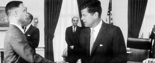 Forrest
Gump shaking hands with J.F.K.
Forrest
Gump shaking hands with J.F.K.
You will be given a working skeleton program, which provides the user interface elements and data structures that you'll need for this program. This skeleton is described below. We have provided a sample solution executable and test images. Try this out to see how your program should run.
Description
This program is based on the paper Intelligent Scissors for Image Composition, by Eric Mortensen and William Barrett, published in the proceedings of SIGGRAPH 1995. The way it works is that the user first clicks on a "seed point" which can be any pixel in the image. The program then computes a path from the seed point to the mouse cursor that hugs the contours of the image as closely as possible. This path, called the "live wire", is computed by converting the image into a graph where the pixels correspond to nodes. Each node is connected by links to its 8 immediate neighbors. Note that we use the term "link" instead of "edge" of a graph to avoid confusion with edges in the image. Each link has a cost relating to the derivative of the image across that link. The path is computed by finding the minimum cost path in the graph, from the seed point to the mouse position. The path will tend to follow edges in the image instead of crossing them, since the latter is more expensive. The path is represented as a sequence of links in the graph.
Next, we describe the details of the cost function and the algorithm for computing the minimum cost path. The cost function we'll use is a bit different than what's described in the paper, but closely matches what was discussed in lecture.
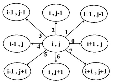
As described in the lecture notes, the image is represented as a graph.
Each pixel (i,j) is represented as a node in the graph, and is connected to its
8 neighbors in the image by graph links (labeled from 0 to 7), as shown in the
following figure.
Cost Function
To simplify the explanation, let's first assume that the image is grayscale instead of color (each pixel has only a scalar intensity, instead of a RGB triple) as a start. The same approach is easily generalized to color images.
- Computing cost for grayscale images
Among the 8 links, two are horizontal (links 0 and 4), two are vertical (links 2 and 6), and the rest are diagonal. The magnitude of the intensity derivative across the diagonal links, e.g. link1, is approximated as:
D(link1)=|img(i+1,j)-img(i,j-1)|/sqrt(2)
The magnitude of the intensity derivative across the horizontal links, e.g.
link 0, is approximated as:
D(link 0)=|(img(i,j-1) + img(i+1,j-1))/2
- (img(i,j+1) + img(i+1,j+1))/2|/2
Similarly, the magnitude of the intensity derivative across the vertical links,
e.g. ln2, is approximated as:
D(link2)=|(img(i-1,j)+img(i-1,j-1))/2-(img(i+1,j)+img(i+1,j-1))/2|/2.
We compute the cost for each link, cost(link), by the following equation:
cost(link)=(maxD-D(link))*length(link)
where maxD is the maximum magnitude of derivatives across links over in the
image, e.g., maxD = max{D(link) | forall link in the image}, length(link) is
the length of the link. For example, length(link 0) = 1, length(link 1) =
sqrt(2) and length(link 2) = 1.
If a link lies along an edge in an image, we expect that the intensity
derivative across that link is large and accordingly, the cost of link is
small.
- Cost for an RGB image
As in the grayscale case, each pixel has eight links. We first compute the magnitude of the intensity derivative across a link, in each color channel independently, denoted as
( DR(link),DG(link),DB(link) ).
Then the magnitude of the color derivative across link is defined as
D(link) = sqrt( (DR(link)*DR(link)+DG(link)*DG(link)+DB(link)*DB(link))/3 ).
Then we compute the cost for link link in the same way as we do for a gray scale image:
cost(link)=(maxD-D(link))*length(link).
Notice that cost(link 0) for pixel (i,j) is the same as cost(link 4) for pixel (i+1,j). Similar symmetry property also applies to vertical and diagonal links.
For debugging perpose, you may want to scale down each link cost by a factor of 1.5 or 2 so that they can be converted to byte format without clamping to[0,255]
- Using cross correlation to compute link intensity derivatives
You are *required* to implement the D(link) formulas above using 3x3 cross correlation. Each of the eight link directions will require using a different cross correlation kernel. You will need to figure out for yourself what the proper entries in each of the eight kernels will be.
Computing the Minimum Cost Path
The pseudo code for the shortest path algorithm in the paper
is a variant of Dijkstra's shortest path algorithm, which is described in any
of the classic algorithm books (including text books used in data structures
courses like 326). You could also refer to any of the classic algorithm
text books (e.g.,
Introduction to Algorithms by Thomas H. Cormen, Charles E. Leiserson, Ronald L.
Rivest, and Cliff Stein, published by MIT Press). Here is some pseudo
code which is equivalent to the algorithm in the SIGGRAPH paper, but we feel is
easier to understand.
procedure LiveWireDP
input: seed, graph
output: a minimum path tree in the input graph with each node
pointing to its predecessor along the minimum cost path to that node from the
seed. Each node will also be assigned a total cost, corresponding to the
cost of the the minimum cost path from that node to the seed.
comment: each node will experience three states: INITIAL, ACTIVE,
EXPANDED sequentially. the algorithm terminates when all
nodes are EXPANDED. All nodes in graph are initialized as INITIAL. When the
algorithm runs, all ACTIVE nodes are kept in a priority queue, pq,
ordered by the current total cost from the node to the seed.
Begin:
initialize the priority queue pq to be empty;
initialize each node to the INITIAL state;
set the total cost of seed to be zero;
insert seed into pq;
while pq is not empty
extract the node q with the minimum total cost in pq;
mark q as EXPANDED;
for each neighbor node r of q
if r has not been EXPANDED
if r is still INITIAL
insert r in pq with the sum of the total cost of q and link cost from q to r as its total cost;
mark r as ACTIVE;
else if r is ACTIVE, e.g., in already in the pq
if the sum of the total cost of q and link cost between q and r is less than the total cost of r
update the total cost of r in pq;
End
We provide the priority queue functions that you will need in the skeleton code (implemented as a binary heap). These are: ExtractMin, Instert, and Update.
Skeleton Code
You can download the skeleton files. The code is compiled in Visual C++ 7.0, and organized by the workspace file iScissor.sln. All the source files (.h/.cpp) are in the subdirectory src. There are 28 files total, but many are just user interface files that are automatically generated by fluid, the FLTK user interface building tool. Here is a description of what's in there:
- ImageLib/*.cpp/h are files taking care of image file I/O. The only image format we support in this tool is targa (.tga) format, which is also readable in Photoshop and most other image viewing and editing tools. One reason we like tga is that it's possible to store a transparency (alpha) channel with the RGB image data, in 32 bit mode. You shouldn't have to change these files.
- IScissorPanelUI.h/cpp, BrushConfigUI.h/cpp, FltDesignUI.h/cpp, ImgFilterUI.h/cpp, and HelpPageUI.h/cpp define four types of windows used in the tool. They are generated by fluid through BrushConfigUI.fl, FltDesignUI.fl, ImgFilterUI.fl, and HelpPageUI.fl. You don't have to worry too much about them if you don't want to change the structures of the windows. If you do decide to change the UI, you may prefer using fluid to do so.
- imgflt.h is a header file used in most of the files.
- FltAux.h defines a few auxiliary structures/routines for the application.
- ImgFltMain.cpp is the main file where you want to start reading.
- correlation.h/cpp are the files where your image filtering code will go.
- ImgView.h/cpp are files where most of the UI requests are implemented. In ImgView.cpp, you want to finish handle() (for extra credit only) so that it applies the brush filter when the left mouse button is pressed and moved.
- PriorityQueue.h, which defines several template classes for dynamic array, binary heap, and doubly linked list. They are useful for representing contours and searching the minimum path tree.
ImgView contains most of the data structures and handles interface messages. You will work with iScissor.cpp most often.
Data structures
The main data structure that you will use in Project 1 is the Pixel Node.
Pixel Node
Use the following Node structure when computing the minimum path tree.
struct
Node{
double linkCost[8];
int state;
double totalCost;
Node *prevNode;
int column, row;
//other unrelated fields;}
linkCost contains the costs of each link, as described above.
state is used to tag the node as being INITIAL, ACTIVE, or EXPANDED during the
min-cost tree computation.
totalCost is the minimum total cost from this node to the seed node.
prevNode points to its predecessor along the minimum cost path from the seed to
that node.
column and row remember the position of the node in original image so that its
neighboring nodes can be located.
For visualization purposes, we provide code to convert a pixel node array into an image that displays the computed cost values in the user interface. This image buffer, called Cost Graph, has the structure shown below. Cost Graph has 3W columns and 3H rows and is obtained by expanding the original image by a factor of 3 in both the horizontal and vertical directions. For each 3 by 3 unit, the RGB(i,j) color is saved at the center and the eight link costs, as described in the Cost Function section, are saved in the 8 corresponding neighbor pixels. The link costs shown are the average of the costs over the RGB channels, as described above (NOT the per-channel costs). The Cost Graph may be viewed as an RGB image in the interface, (dark = low cost, light = high cost).
|
|
|
|||||||||||||||||||||||||||
|
|
|
|||||||||||||||||||||||||||
|
|
|
|||||||||||||||||||||||||||
|
Pixel layout in Cost Graph (3W*3H) |
|||||||||||||||||||||||||||||
User Interface
File-->Save Contour, save image with contour marked;
File-->Save Mask, save compositing mask for PhotoShop;
Tool-->Scissor, open a panel to choose what to draw in the window
Work Mode:
Image Only: show original image without contour superimposed on it;
Image with Contour: show original image with contours superimposed on it;
Debug Mode:
Pixel Node: Draw a cost graph with original image pixel colors at the center of each 3by3 window, and black everywhere else;
Cost Graph: Draw a cost graph with both pixel colors and link costs, where you can see whether your cost computation is reasonable or not, e.g., low cost (dark intensity) for links along image edges.
Path Tree: show minimum path tree in the cost graph for the current seed; You can use the counter widget to simulate how the tree is computed by specifying the number of expanded nodes. The tree consists of links with yellow color. The back track direction (towards the seed) goes from light yellow to dark yellow.
Min Path: show the minimum path between the current seed and the mouse position;
Ctrl+"+", zoom in;
Ctrl+"-", zoom out;
Ctrl+Left click first seed;
Left click, following seeds;
Enter, finish the current contour;
Ctrl+Enter, finish the current contour as closed;
Backspace, when scissoring, delete the last seed; otherwise, delete selected contour.
Select a contour by moving onto it. Selected contour is red, un-selected ones are green.
To Do
All the required work can be done in iScissor.cpp, iScissor.h, and correlation.cpp.
1. implement InitNodeBuf, which takes as input an image of size W by H and an allocated node buffer of the same dimensions, and initializes the column, row, and linkCost fields of each node in the buffer. InitNodeBuf MUST make calls to pixel_filter.You will also need to modify the eight cross correlation kernels defined in iScissor.h.
2. implement pixel_filter, which takes as input an image of size W by H, a filter kernel, and a pixel position at which to compute the cross correlation.
3. implement image_filter, which applies a filter to an entire image. You may do this by making calls to pixel_filter if you wish.
4. implement LiveWireDP, which takes a node buffer and a seed position as input and computes the minimum path tree from the seed node.
5. implement MinimumPath, which takes as input a node buffer and a node position and returns a list of nodes along the minimum cost path from the input node to the seed node in the buffer (the seed has a NULL predecessor).
The Artifact
For this assignment, you will turn in a final image (the artifact) which is a composite created using your program. Your composite can be derived from as many different images as you'd like. Make it interesting in some way--be it humorous, thought provoking, or artistic! You should use your own scissoring tool to cut the objects out and save them to matte files, but then can use Photoshop or any other image editing program to process the resulting mattes (move, rotate, adjust colors, warp, etc.) and combine them into your composite. Instructions on how to do this in Photoshop are provided here. You should still turn in an artifact even if you don't get the program working fully, using the scissoring tool in the sample solution or in Photoshop.
Besides the artifact, please also turn in a web-page that includes all your original images, all the masks you made, and a description of the process, including anything special you did. The web-page should be placed in the project1/artifact directory along with all the images in JPEG format. If you are unfamiliar with HTML you can use any web-page editor such as FrontPage, Word, or Visual Studio 7.0 to make your web-page.
The class will vote on the best composites.
Bells and Whistles
Here is a list of suggestions for extending the program for extra credit. You are encouraged to come up with your own extensions. We're always interested in seeing new, unanticipated ways to use this program!
![]() One
problem with the live wire is that it prefers shorter paths so will tend to cut
through large object rather than wrap around them. One way to fix this is
specify a specific region in which the path must stay. As long as this
region contains the object boundary but excludes most of the interior, the path
will be forced to follow the boundary. One way of specifying such a
region is to use a thick (e.g., 50 pixel wide) paint brush. Implement
this feature. Note: we already provide support for brushing a
region using a selection buffer.
One
problem with the live wire is that it prefers shorter paths so will tend to cut
through large object rather than wrap around them. One way to fix this is
specify a specific region in which the path must stay. As long as this
region contains the object boundary but excludes most of the interior, the path
will be forced to follow the boundary. One way of specifying such a
region is to use a thick (e.g., 50 pixel wide) paint brush. Implement
this feature. Note: we already provide support for brushing a
region using a selection buffer.
![]() Modify
the interface and program to allow blurring the image by different amounts
before computing link costs. Describe your observations on how this
changes the results.
Modify
the interface and program to allow blurring the image by different amounts
before computing link costs. Describe your observations on how this
changes the results.
![]() Try
different costs functions, for example the method described in
Intelligent Scissors for Image Composition, and modify the user
interface to allow the user to select different functions. Describe
your observations on how this changes the results.
Try
different costs functions, for example the method described in
Intelligent Scissors for Image Composition, and modify the user
interface to allow the user to select different functions. Describe
your observations on how this changes the results.
![]() The
only point that doesn't snap to edges is the seed. Implement a seed
snapping feature, where the seed is automatically moved to the closest edge.
The
only point that doesn't snap to edges is the seed. Implement a seed
snapping feature, where the seed is automatically moved to the closest edge.
![]() Implement
path cooling, as described in
Intelligent Scissors for Image Composition.
Implement
path cooling, as described in
Intelligent Scissors for Image Composition.
![]()
![]() Implement
dynamic training, as described in
Intelligent Scissors for Image Composition.
Implement
dynamic training, as described in
Intelligent Scissors for Image Composition.
Add other interesting editing operations--see here for some inspiring examples (credit depends on what you implement!)
![]()
![]() Implement
a live wire with sub-pixel precision. You can find the position of
an edge to sub-pixel precision by
fitting a curve (e.g., a parabola) to the gradient magnitude values
across an edge, and finding the maximum. Another way (more complex but
potentially better) of doing this is given in a
follow on to Mortensen's scissoring paper. It is probably easiest
to first compute the standard (pixel-precision) live wire and then use one of
these curve fitting techniques to refine it.
Implement
a live wire with sub-pixel precision. You can find the position of
an edge to sub-pixel precision by
fitting a curve (e.g., a parabola) to the gradient magnitude values
across an edge, and finding the maximum. Another way (more complex but
potentially better) of doing this is given in a
follow on to Mortensen's scissoring paper. It is probably easiest
to first compute the standard (pixel-precision) live wire and then use one of
these curve fitting techniques to refine it.
?/span>
Last modified on September 30, 2003