Introduction

Caustics are generated in nature when light is refocused by a reflective or refractive surface. Good everyday examples of caustics include the light patterns on the bottom of a swimming pool and the intense spot of light that results from holding a magnifying glass up to the sun. You can also observe caustics the next time you have a pint of beer by looking at the patterns of light in the shadow of your glass.

Standard ray tracing techniques are unable to simulate caustics. Instead, we need to trace the path of photons from light sources as they traverse the scene and model the effect of refractive and reflective surfaces. Photon Mapping, as described by Jensen [1], provides an efficient and straightforward method for tracing, tracking, and recovering photons in a scene.

Our final project implemented this photon mapping technique on top of the CSE557 ray tracer code. We succeeded in generating a number of realistic caustics, shown below in the results section.

Photon Map Data Structure

Our data structure for a photon contains the position, incident direction, power, and color of the given photon. Our photon map is essentially a modified version of a BSP tree. We choose this representation (as opposed to the k-d tree employed by Jensen [1]) because we already had an implementation of a BSP tree from our ray tracer’s acceleration code. The primary difference between our BSP tree and the k-d tree is that in the BSP tree, photons are only stored in the leaf nodes. In creating the BSP tree, when splitting a node into its two children, we compute the average value of the coordinate of the splitting plane of the photons in the node. This value is then used to determine the location of the splitting plane in the hopes that a roughly equal number of photons will be placed in the two children nodes, resulting in a relatively balanced tree.

Mapping the Photons

Immediately after loading a scene into the ray tracer, our implementation creates the photon map. We do this by looping through all of the light sources in the scene, and for each light source, tracing a large (and UI controlled) number of photons from the light source into the scene. For point lights we use the method described in Jensen’s book [1]. Specifically, we first compute a unit sphere enclosing the point light. We then embed this sphere inside a bounding cube and generate random points inside the cube. For every randomly generated point that also lands inside the sphere, we use this point as the direction for an emitted photon, and trace this photon into the scene. The case of directional lights is a bit more complicated. Jensen [1] provides a high-level overview of the technique, which we adapted to work with our ray tracer. We begin by computing a bounding sphere that encloses the entire scene. We then project this sphere onto a plane that is orthogonal to the direction of the light source. Using a similar technique to that employed for point lights, we compute a bounding square around the projected circle on the plane, generate random points inside the square, and for each point that lands inside the circle, we trace a photon into the scene from that point with direction equal to that of the directional light. These randomized techniques allow us to efficiently achieve a roughly uniform distribution of photons over directions in the case of point lights, and over points of origin in the case of directional lights.

To actually trace an emitted photon, we once again use a method from Jensen’s book [1]. We have a routine that is very similar in structure to the standard ray tracing routine, but with one major difference. Whenever a photon intersects an object in the scene, we use a probabilistic method known as “Russian Roulette” to determine whether the photon is absorbed, reflected, or refracted. The probabilities of reflection and refraction are proportional to the percentage of the incoming light that would be allocated to the corresponding ray in a traditional ray tracer. If the photon is absorbed, we update the photon’s fields accordingly and add the photon to a global list that maintains all of the photons deposited in the scene. We use recursive calls to the trace photon routine to handle the cases where the photon is reflected or refracted. When a photon is reflected or refracted by a material which has non-uniform values for the R, G and B components of its reflectivity or transmissiveness, we scale the RGB components of the reflected or refracted photon proportionally.

Finally, after all of the emitted photons have been traced in the scene, we build the photon map BSP tree from the global list of photons.

Estimating Radiosity

Once we have completed the photon map, we proceed with traditional ray tracing, sending view rays from the camera into the scene and reflecting and refracting the rays when they intersect objects. In the Phong shading routine, we follow Jensen’s suggestion [1] again and calculate the illumination at the point of intersection by calculating an estimate of the local photon flux. This flux calculation replaces the casting of shadow rays toward light sources found in ray tracers without photon mapping. The flux calculation takes into account the angle between the material’s normal at the point of intersection and the photon's incident direction, allowing us to model specular highlights and the effect of light angle on diffuse shading.

The flux estimate is based on the nearest N photons, where N is a pre-specified parameter, typically on the order of one or two hundred photons. To find the nearest N photons, we adapted Jensen's algorithm [1] to work with BSP trees, rather than k-d trees. The nearest-neighbors algorithm keeps track of a maximum distance d to the intersection point. We begin the search at the root node, and recursively search the child node whose bounding box contains the intersection point. Once we return from the recursive search, we search the other child node if and only if its bounding box intersects a sphere centered at the intersection point with radius equal to the current value of d. When we reach the leaf nodes, we add any photons found within distance d of the intersection point to a priority queue keyed on the distance between the photon and the intersection point. If the addition of a new photon causes the size of the priority queue to be greater than N, we remove the maximum distance photon from the queue and set d to the distance of the new maximum distance photon in the queue. By decreasing the value of d we can prune some unnecessary branches from the tree search.

Once we have found the N nearest photons, we estimate the flux using the following formula, from Jensen’s text [1]:

Where r is the distance to the N-th nearest photon, f(x,w,d_p) is the equation for specular and diffuse shading at a point x with view ray direction w and incoming light direction d_p, and is the power of photon p. Notice that this formula allows us to calculate each photon's individual contribution to the diffuse and specular shading in terms of its power and direction, and to simply sum the contributions up at the end and divide the result by 2πr².

Results

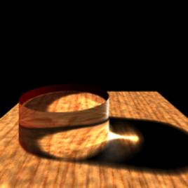
The four images above show examples of caustics generated by our photon mapping ray tracer. All four images were generated by sending 1,000,000 photons from a directional light towards a table with a glass object resting on top. We estimated the local photon flux at each point using the 100 nearest photons in the map. The first three scenes contain simple geometric objects – a cone, a sphere, and a cylinder. The fourth contains a chess piece created using a triangular mesh.

The image above is a link to an animation showing the caustics generated by a light moving through an otherwise fixed scene. We moved the light in a circle around the cylinder, varied its elevation sinusoidally, and twice varied the width of the light beam. For the animation, we used 2,000,000 photons and estimated the local flux using the 200 nearest neighbors in order to reduce the brightness variations.

References

[1] Jensen, Henrik W. Realistic Image Synthesis Using Photon Mapping. Natick, MA: AK Peters, Ltd. 2001.