Project 3: Animator
|
Assigned Date : 2/20/2008 |
|
Project 3: Animator
|
This project consists of three parts: (1) use a simple OpenGL modeling tool to create and animate the hierarchical models of your own design (2) compose them into a scene and implement a keyframe animation system and (3) implement a particle system and integrate it with the animation system. We have provided a nifty user interface to help you draw curves and animate your model. When finished with the coding part of the project, you will use your system to create an animation artifact.
A hierarchical model is a way of grouping together shapes and attributes to form a complex object. Parts of the object are defined in relationship to each other as opposed to their position in some absolute coordinate system. Think of each object as a tree, with nodes decreasing in complexity as you move from root to leaf. Each node can be treated as a single object, so that when you modify a node you end up modifying all its children together. Hierarchical modeling is a very common way to structure 3D scenes and objects, and is found in many other contexts. We provide a simple framework such that you can experiment your hierarchical model.
First of all, you must come up with a character. This character can be composed solely of primitive shapes (box, generalized cylinder, sphere, and triangle). It should use at least ten primitives and at least four levels of hierarchy. You must also use at least one each of the glTranslate(), glRotate() and glScale() calls to position these primitives in space (and you will probably use many of all of them!) You must also use glPushMatrix() and glPopMatrix() to nest your matrix transformations. The modeler skeleton provides functions for creating sliders and hooking them to different features of your model. You must add at least one of these as a control knob (slider, actually) for some joint/component of your model - have your character do some simple action as you scrub a slider back and forth. In addition, at least one of your controls must be tied to more than one joint/component; this knob will change the input to some function that determines how several parts of your model can move. For example, in a model of a human, you might have a slider that straightens a leg by extending both the knee and hip joints.
Keyframe animation is one of the most common methods for controlling a hierarchical model. The idea is to pose the model at select moments in time and then smoothly interpolate between the poses (sometimes called "in-betweening"). The pose is determined by the control parameters (degrees of freedom) of the model, such as joint angles, and each parameter has a separate curve describing how it changes over time. In practice, you do not need to pose the whole model at each keyframe; you can adjust each curve independently, adding keyframes for that curve as needed. For this component of the project, you will implement a set of curve types for keyframe interpolation.
You will need to implement each of the following curve types:
- B�zier (splined together with C0 continuity)
- Catmull-Rom
- B-spline
The GraphWidget object owns a bunch of Curve objects. The Curve class is used to represent the time-varying splines associated with your model parameters. You don't need to worry about most of the existing code, which is used to handle the spiffy user interface. The one important thing to understand is the curve evaluation model. Each curve is represented by a vector of control points, and a vector of evaluated points.
mutable std::vector
mutable std::vector
Control points define a curve; they are the ones that you can see and manipulate in the graph interface. The evaluated points are a sampled representation of the curve itself (i.e. the solid line that runs through or near the control points). At any given time t, the value of the curve is defined as the interpolated value between the two closest evaluated points (i.e. the two evaluated points on either side of t).
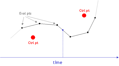
Since the user only specifies control points in the graph widget, the program must determine the actual shape of the curve. In other words, given a set of control points, the system figures out what the evaluated points are. This conversion process is handled by the CurveEvaluator member variable of each curve.
const CurveEvaluator* m_pceEvaluator;
In the skeleton, we've only implemented the LinearEvaluator. You should use this as a model to implement the other types of curve evaluators required: B�zier, B-Spline, and Catmull-Rom. The following section describes in greater detail what you need to do to add a curve.
For each curve type, you must write a new class derived from CurveEvaluator. Inside the class, you should implement the evaluateCurve function. This function takes the following parameters: ptvCtrlPts--a collection of control points that you specify in the curve editor, ptvEvaluatedCurvePts--a collection of evaluated curve points that you return from the function calculated using the curve type's formulas, fAniLength (the maximum time that a curve is defined), and bWrap - a flag indicating whether or not the curve should be wrapped. To add a new curve type, you should look in the GraphWidget constructor and change the following lines to use your new set of evaluator classes.
m_ppceCurveEvaluators[CURVE_TYPE_BSPLINE]
= new LinearCurveEvaluator();
m_ppceCurveEvaluators[CURVE_TYPE_BEZIER] = new LinearCurveEvaluator();
m_ppceCurveEvaluators[CURVE_TYPE_CATMULLROM] = new LinearCurveEvaluator();
For B�zier curves (and the splines based on them), it is sufficient to sample the curve at fixed intervals of time. The adaptive de Casteljau subdivision algorithm presented in class may be implemented for an extra bell.
You do not have to sort the control points or the evaluated curve points. This has been done for you. Note, however, that for an interpolating curve (Catmull-Rom), the fact that the control points are given to you sorted by x does not ensure that the curve itself will also monotonically increase in x. You should recognize and handle this case appropriately. One solution is to return only the evaluated points that are increasing monotonically in x.
The skeleton code has a very high-level framework in place for running particle simulations that is based on Witkin's Particle System Dynamics paper in the course reader. In this model, there are three major components:
You are responsible for coming up with a representation for particles and forces.
Here are the specific requirements for the particle system:
Once you've completed these tasks, you should be able to run your particle system simulation by playing your animation with the "Simulate" button turned on. As you simulate, the position of the particles at each time step are baked so that you can replay your animation without re-simulating. When you disable simulation, normal animation continues. The gray region in the white indicator window above the time slider indicates the time for which the simulation has been "baked."
The skeleton provides a very basic outline of a simulation engine, encapsulated by the ParticleSystem class. Currently, the header file (ParticleSystem.h) specifies an interface that must be supported in order for your particle system to interact correctly with the animator UI. Alternately, you can try to figure out how the UI works yourself by searching within the project files for all calls to the particle system's functions, and then re-organizing the code. This second option may provide you with more flexibility in doing some very ambitious particle systems with extra UI support. However, the framework seems general enough to support a wide range of particle systems. There is detailed documentation in the header file itself that indicates what each function you are required to write should do. Note that the ParticleSystem declaration is by no means complete. As mentioned above, you will have to figure out how you want to store and organize particles and forces, and as a result, you will need to add member variables and functions.
One of the functions you are required to implement is called computeForcesAndUpdateParticles:
virtual void computeForcesAndUpdateParticles(float t);
This function represents the meat of the simulation solver. Here you will compute the forces acting on each particle and update their positions and velocities based on these forces using Euler's method. As mentioned above, you are responsible for modeling particles and forces in some way that allows you to perform this update step at each frame.
In the sample robotarm.cpp file, there is a comment in the main function that indicates where you should create your particle system and hook it up into the animator interface. After creating your ParticleSystem object, you should do the following:
ParticleSystem *ps = new ParticleSystem();
...
// do some more particle system setup
...
ModelerApplication::Instance()->SetParticleSystem(ps);
The interface for this project consists of two components: a slider control interface and an animation curve interface. The slider control interface allows you to control each degree of freedom of your hierachical model with a slider. The animation curve interface allows you to specify how each degree of freedom behaves as a function of time. In addition, you can manipulate the viewpoint by interacting directly with the view of the 3D model.
In the skeleton code distribution, we've included the fluid file for the ModelerUIWindows class (modeleruiwindows.fl). In addition, we've included the binary for fluid so that you can (if you want) make additions to the UI.
After selecting a series of model parameters in the browser window, their corresponding animation curves are displayed in the graph. Each spline is evaluated as a simple piece-wise linear curve that linearly interpolates between control points. You can manipulate the curves as follows:
|
Command |
Action |
| LEFT MOUSE | Clicking anywhere in the graph creates a control point for the selected curve. Ctrl points can be moved by clicking on them and dragging. |
| CTRL LEFT MOUSE | Selects the curve |
| SHIFT LEFT MOUSE | Removes a control point |
| ALT LEFT MOUSE | Rubber-band selection of control points |
| RIGHT MOUSE | Zooms in X and Y dimensions |
| CTRL RIGHT MOUSE | Zooms into the rubber-banded space region |
| SHIFT RIGHT MOUSE | Pans the viewed region |
Note that each of the displayed curves has a different scale. Based on the maximum and minimum values for each parameter that you specified in your model file, the curve is drawn to "fit" into the graph. You'll also notice that the other curve types in the drop-down menu are not working. One part of your requirements (outlined below) is to implement these other curves.
At the bottom of the window is a simple set of VCR-style controls and a time slider that let you view your animation. "Loop" will make the animation start over when it reaches the end. The "Simulate" button relates to the particle system which is discussed below. You can use the Camera keyframing controls to define some simple camera animations. When you hit "Set", the current camera position and orientation (pose) is saved as a keyframe. By moving the time slider and specifying different pose keyframes, the camera will linearly interpolate between these poses to figure out where it should be at any given time. You can snap to a keyframe by clicking on the blue indicator lines, and if you hit "Remove", the selected keyframe will be deleted. "Remove All" removes all keyframes.
You will eventually use the curve editor and the particle system simulator to produce an animated artifact for this project. Under the File menu of the program, there is a Save Movie As option, that will let you specify a base filename for a set of movie frames. Each frame is saved as a bitmap.
Each group should turn in their own artifact. We may give extra credit to those that are exceptionally clever or aesthetically pleasing. Try to use the ideas discussed in the John Lasseter article in your CoursePak. These include anticipation, follow-through, squash and stretch, and secondary motion.
Finally, please try to limit your animation to 30 seconds or less. This may seem like a short amount of time, but it really isn't. Frequently, animations that are longer than this time seem to be running in slow motion. Actions should be quick and to the point.
![]() Render your particle system as something other than white points!
Render your particle system as something other than white points!
![]() Particles rendered as points or spheres may not look that realistic. You can achieve more
spectacular effects with a simple technique called billboarding. A
billboarded quad (aka "sprite") is a textured square that always
faces the camera. See the
sprites demo. For full credit, you should load a texture with
transparency (sample textures), and
turn on alpha blending (see this tutorial
for more information). Hint: When rotating your particles to face the
camera, it's helpful to know the camera's up and right vectors in
world-coordinates.
Particles rendered as points or spheres may not look that realistic. You can achieve more
spectacular effects with a simple technique called billboarding. A
billboarded quad (aka "sprite") is a textured square that always
faces the camera. See the
sprites demo. For full credit, you should load a texture with
transparency (sample textures), and
turn on alpha blending (see this tutorial
for more information). Hint: When rotating your particles to face the
camera, it's helpful to know the camera's up and right vectors in
world-coordinates.
![]() Use the billboarded quads you implemented above to render the following effects.
Each of these effects is worth one whistle provided you have put in a whistle
worth of effort making the effect look good.
Use the billboarded quads you implemented above to render the following effects.
Each of these effects is worth one whistle provided you have put in a whistle
worth of effort making the effect look good.
glBlendFunc(GL_SRC_ALPHA,GL_ONE);)
![]() Render a mirror in your scene. As you may already know, OpenGL has no built-in reflection
capabilities. You can simulate a mirror with the following steps: 1) Reflect
the world about the mirror's plane, 2) Draw the reflected world, 3) Pop the
reflection about the mirror plane from your matrix stack, 4) Draw your world as
normal. After completing these steps, you may discover that some of the
reflected geometry appears outside the surface of the mirror. For an
extra whistle you can clip the reflected image to the mirror's surface, you
need to use something called the stencil buffer. The stencil buffer is
similar to a Z buffer and is used to restrict drawing to certain portions of
the screen. See Scott Schaefer's
site for more information. In addition, the NeHe game development site has
a detailed tutorial
Render a mirror in your scene. As you may already know, OpenGL has no built-in reflection
capabilities. You can simulate a mirror with the following steps: 1) Reflect
the world about the mirror's plane, 2) Draw the reflected world, 3) Pop the
reflection about the mirror plane from your matrix stack, 4) Draw your world as
normal. After completing these steps, you may discover that some of the
reflected geometry appears outside the surface of the mirror. For an
extra whistle you can clip the reflected image to the mirror's surface, you
need to use something called the stencil buffer. The stencil buffer is
similar to a Z buffer and is used to restrict drawing to certain portions of
the screen. See Scott Schaefer's
site for more information. In addition, the NeHe game development site has
a detailed tutorial
![]() Use environment mapping to simulate a reflective material. This technique is particularly
effective at faking a metallic material or reflective, rippling water
surface. Note that OpenGL provides some very useful functions for
generating texture coordinates for spherical environment mapping. Part of
the challenge of this whistle is to find these functions and understand how
they work.
Use environment mapping to simulate a reflective material. This technique is particularly
effective at faking a metallic material or reflective, rippling water
surface. Note that OpenGL provides some very useful functions for
generating texture coordinates for spherical environment mapping. Part of
the challenge of this whistle is to find these functions and understand how
they work.
![]() Implement a motion blur effect (example). The easy
way to implement motion blur is using an accumulation
buffer - however, consumer grade graphics cards do not implement an
accumulation buffer. You'll need to simulate an accumulation buffer by
rendering individual frames to a texture, then combining those textures.
See this
tutorial for an example of rendering to a texture.
Implement a motion blur effect (example). The easy
way to implement motion blur is using an accumulation
buffer - however, consumer grade graphics cards do not implement an
accumulation buffer. You'll need to simulate an accumulation buffer by
rendering individual frames to a texture, then combining those textures.
See this
tutorial for an example of rendering to a texture.
![]() Use a texture map on all or part of your character. (The safest way to do this is to implement your own primitives inside your model file that do texture mapping.)
Use a texture map on all or part of your character. (The safest way to do this is to implement your own primitives inside your model file that do texture mapping.)
![]() Build a complex shape as a set of polygonal faces, using triangles (either the provided primitive or straight OpenGL triangles) to render it.
Examples of things that don't count as complex: a pentagon, a square, a circle. Examples of what does count: dodecahedron, 2D function plot (z = sin(x2 + y)), etc.
Build a complex shape as a set of polygonal faces, using triangles (either the provided primitive or straight OpenGL triangles) to render it.
Examples of things that don't count as complex: a pentagon, a square, a circle. Examples of what does count: dodecahedron, 2D function plot (z = sin(x2 + y)), etc.
![]() Heightfields are great ways to build complicated looking maps and terrains pretty easily.
Heightfields are great ways to build complicated looking maps and terrains pretty easily.
![]() Add a lens flare. This effect has components both in screen space and world
space effect.
For full credit, your lens flare should have at least 5 flare
"drops", and the transparency of the drops should change depending on
how far the light source is from the center of the screen. You do not
have to handle the case where the light source is occluded by other geometry
(but this is worth an extra whistle).
Add a lens flare. This effect has components both in screen space and world
space effect.
For full credit, your lens flare should have at least 5 flare
"drops", and the transparency of the drops should change depending on
how far the light source is from the center of the screen. You do not
have to handle the case where the light source is occluded by other geometry
(but this is worth an extra whistle).
![]() If you find something you don't like about the
interface, or something you think you could do better, change it! Any
really good changes will be incorporated into Animator 2.0. Credit
varies with the quality of the improvement.
If you find something you don't like about the
interface, or something you think you could do better, change it! Any
really good changes will be incorporated into Animator 2.0. Credit
varies with the quality of the improvement.
![]()
![]() Add a function in your model file for drawing a new type of primitive. The following examples will definitely garner two bells; if you come up with your own primitive, you will be awarded one or two bells based on its coolness.
Here are three examples:
Add a function in your model file for drawing a new type of primitive. The following examples will definitely garner two bells; if you come up with your own primitive, you will be awarded one or two bells based on its coolness.
Here are three examples:
![]()
![]() Use some sort of procedural modeling (such as an L-system) to generate all or part of your character
or to create a new model for your scene. Have parameters of the procedural modeler controllable by the user via control widgets.
Use some sort of procedural modeling (such as an L-system) to generate all or part of your character
or to create a new model for your scene. Have parameters of the procedural modeler controllable by the user via control widgets.
![]()
![]() If you implemented a "twist" degree of freedom for some
part of your model, applying the rotational degrees of freedom can give some unexpected results. For
example, twist your the degree of freedom by 90 degrees. Now try to do rotations as
normal. This effect is called gimbal lock. Implement Quaternions as a method for avoiding the
gimbal lock.
If you implemented a "twist" degree of freedom for some
part of your model, applying the rotational degrees of freedom can give some unexpected results. For
example, twist your the degree of freedom by 90 degrees. Now try to do rotations as
normal. This effect is called gimbal lock. Implement Quaternions as a method for avoiding the
gimbal lock.
![]()
![]() Implement picking of a part in the model
hierarchy. In other words, make it so that you can click on a part
of your model to select its animation curve. To recognize which body
part you're picking, you need to first render all body parts into a hidden
buffer using only an emissive color that corresponds to an object
ID. After modifying the mouse-ing UI to know about your new picking
mode, you'll figure out which body part the user has picked by reading out
the ID from your object ID buffer at the location where the mouse
clicked. This should then trigger the GraphWidget to select
the appropriate curve for editing. If you're thinking of doing
either of the six-bell inverse kinematics (IK) extensions below, this kind
of interface would be required.
Implement picking of a part in the model
hierarchy. In other words, make it so that you can click on a part
of your model to select its animation curve. To recognize which body
part you're picking, you need to first render all body parts into a hidden
buffer using only an emissive color that corresponds to an object
ID. After modifying the mouse-ing UI to know about your new picking
mode, you'll figure out which body part the user has picked by reading out
the ID from your object ID buffer at the location where the mouse
clicked. This should then trigger the GraphWidget to select
the appropriate curve for editing. If you're thinking of doing
either of the six-bell inverse kinematics (IK) extensions below, this kind
of interface would be required.
![]()
![]()
![]() Implement projected textures.
Projected textures are used to simulate things like a slide projector,
spotlight illumination, or casting shadows onto arbitrary geometry. Check
out this demo and read details
of the effect at glBase,
and SGI.
Implement projected textures.
Projected textures are used to simulate things like a slide projector,
spotlight illumination, or casting shadows onto arbitrary geometry. Check
out this demo and read details
of the effect at glBase,
and SGI.
![]()
![]()
![]() One difficulty with hierarchical modeling using primitives is the difficulty of building "organic" shapes.
It's difficult, for instance, to make a convincing looking human arm because you can't really show the bending of the skin and bulging of the muscle using cylinders and spheres.
There has, however, been success in building organic shapes using metaballs.
Implement your hierarchical model and "skin" it with metaballs. Hint: look up "marching cubes" and "marching tetrahedra" --these are two commonly used algorithms for volume rendering.
For an additional bell, the placement of the metaballs should depend on some sort of interactically controllable hierarchy.
Try out a demo application.
One difficulty with hierarchical modeling using primitives is the difficulty of building "organic" shapes.
It's difficult, for instance, to make a convincing looking human arm because you can't really show the bending of the skin and bulging of the muscle using cylinders and spheres.
There has, however, been success in building organic shapes using metaballs.
Implement your hierarchical model and "skin" it with metaballs. Hint: look up "marching cubes" and "marching tetrahedra" --these are two commonly used algorithms for volume rendering.
For an additional bell, the placement of the metaballs should depend on some sort of interactically controllable hierarchy.
Try out a demo application.
Metaball Demos:These demos show the use of metaballs within the modeler framework. The first demo allows you to play around with three metaballs just to see how they interact with one another. The second demo shows an application of metaballs to create a twisting snake-like tube. Both these demos were created using the metaball implementation from a past CSE 457 student's project.
Demo 1: Basic Texture Mapped Metaballs
Demo 2: Cool Metaball Snake
![]()
![]()
![]()
![]() Another method to build organic shapes is subdivision surfaces.
Implement these for use in your model. You may want to visit this to get some starter code.
Another method to build organic shapes is subdivision surfaces.
Implement these for use in your model. You may want to visit this to get some starter code.
![]()
![]()
![]()
![]()
![]()
![]() Extend your system to support subdivision surfaces. Provide a simple
interface for the user to edit a surface. The user should also be
able to specify surface features that stay constant so that sharp creases
can be formed. Tie your surface to the animation curves to
demonstrate a dynamic scene. Look
Extend your system to support subdivision surfaces. Provide a simple
interface for the user to edit a surface. The user should also be
able to specify surface features that stay constant so that sharp creases
can be formed. Tie your surface to the animation curves to
demonstrate a dynamic scene. Look
![]() The linear curve code provided in the skeleton can be "wrapped,"
which means that the curve has C0 continuity between the end of
the animation and the beginning. As a result, looping the animation
does not result in abrupt jumps. To get credit for wrapping, you must
implement it for each curve type; for information on B�zier curve wrapping,
please click here or for more information in general
look here.
The linear curve code provided in the skeleton can be "wrapped,"
which means that the curve has C0 continuity between the end of
the animation and the beginning. As a result, looping the animation
does not result in abrupt jumps. To get credit for wrapping, you must
implement it for each curve type; for information on B�zier curve wrapping,
please click here or for more information in general
look here.
![]() Enhance the required spline options. Some of these will
require alterations to the user interface, which is somewhat complicated
to understand. If you want to access mouse events in the graph
window, look at the handle function in the GraphWidget
class. Also, look at the Curve class to see what control
point manipulation functions are already provided. These could be
helpful, and will likely give you a better understanding of how to modify
or extend your program's behavior. A maximum of 3 whistles will be
given out in this category.
Enhance the required spline options. Some of these will
require alterations to the user interface, which is somewhat complicated
to understand. If you want to access mouse events in the graph
window, look at the handle function in the GraphWidget
class. Also, look at the Curve class to see what control
point manipulation functions are already provided. These could be
helpful, and will likely give you a better understanding of how to modify
or extend your program's behavior. A maximum of 3 whistles will be
given out in this category.
![]() Implement adaptive B�zier curve generation; i.e., use
a recursive, divide-and-conquer, de Casteljau algorithm to produce
B�zier curves, rather than just sampling them at some arbitrary
interval. You are required to provide some way to change these variables,
with a keystroke or mouse click. In addition, you should have some
way of showing (a printf statement is fine) the number of points
generated for a curve to demonstrate your adaptive algorithm at
work. If you provide visual controls to toggle the feature, modify
the flatness parameter (with a slider for e.g.) and show the number of
points generated for each curve, you will get an extra whistle.
Implement adaptive B�zier curve generation; i.e., use
a recursive, divide-and-conquer, de Casteljau algorithm to produce
B�zier curves, rather than just sampling them at some arbitrary
interval. You are required to provide some way to change these variables,
with a keystroke or mouse click. In addition, you should have some
way of showing (a printf statement is fine) the number of points
generated for a curve to demonstrate your adaptive algorithm at
work. If you provide visual controls to toggle the feature, modify
the flatness parameter (with a slider for e.g.) and show the number of
points generated for each curve, you will get an extra whistle.
![]() Implement a "general" subdivision curve, so the
user can specify an arbitrary averaging mask. You will receive still
more credit if you can generate, display, and apply the evaluation masks
as well. There's a
Implement a "general" subdivision curve, so the
user can specify an arbitrary averaging mask. You will receive still
more credit if you can generate, display, and apply the evaluation masks
as well. There's a
![]()
![]() Implement a C2-Interpolating curve. There is
already an entry for it in the drop-down menu. See write-up from the Bartels,
Beatty, and Barsky book (in the course reader).
Implement a C2-Interpolating curve. There is
already an entry for it in the drop-down menu. See write-up from the Bartels,
Beatty, and Barsky book (in the course reader).
![]()
![]() Add the ability to edit Catmull-Rom curves using the two
"inner" B�zier control points as "handles" on the interpolated
"outer" Catmull-Rom control points. After the user tugs on handles, the
curve will, in general, no longer be Catmull-Rom. In other words, the user
starts by drawing a C1 continuous curve with the
Catmull-Rom choice for the inner B�zier points, but can then be modified
by selecting and editing the handles. The user should be
allowed to drag the interpolated point in a manner that causes the inner
B�zier points to be dragged along. See PowerPoint and
Illustrator pencil-drawn curves for an example. Credit will vary depending
on how much freedom the user is given to edit the inner control points; e.g.,
Powerpoint allows you to constrain the inner control points to make the curve C1
("Smooth"), G1 ("Straight"), or C0/G0
("Corner") around the interpolated point. More credit is available if
you can make the curve C-1, which would allow you, for example, to do
camera jump-cuts easily.
Add the ability to edit Catmull-Rom curves using the two
"inner" B�zier control points as "handles" on the interpolated
"outer" Catmull-Rom control points. After the user tugs on handles, the
curve will, in general, no longer be Catmull-Rom. In other words, the user
starts by drawing a C1 continuous curve with the
Catmull-Rom choice for the inner B�zier points, but can then be modified
by selecting and editing the handles. The user should be
allowed to drag the interpolated point in a manner that causes the inner
B�zier points to be dragged along. See PowerPoint and
Illustrator pencil-drawn curves for an example. Credit will vary depending
on how much freedom the user is given to edit the inner control points; e.g.,
Powerpoint allows you to constrain the inner control points to make the curve C1
("Smooth"), G1 ("Straight"), or C0/G0
("Corner") around the interpolated point. More credit is available if
you can make the curve C-1, which would allow you, for example, to do
camera jump-cuts easily.
![]() Modify your particle system so that the particles' velocities gets initialized with the
velocity of the hierarchy component from which they are emitted. The particles
may still have their own inherent initial velocity. For example, if your model
is a helicopter with a cannon launching packages out if it, each package's
velocity will need to be initialized to the sum of the helicopter's velocity
and the velocity imparted by the cannon.
Modify your particle system so that the particles' velocities gets initialized with the
velocity of the hierarchy component from which they are emitted. The particles
may still have their own inherent initial velocity. For example, if your model
is a helicopter with a cannon launching packages out if it, each package's
velocity will need to be initialized to the sum of the helicopter's velocity
and the velocity imparted by the cannon.
![]() Euler's method is a very simple technique for solving the system of differential equations that
defines particle motion. However, more powerful methods can be used to
get better, more accurate results. Implement your simulation engine using
a higher-order method such as the Runge-Kutta technique. ( Numerical Recipes,
Sections 16.0, 16.1) has a description of Runge-Kutta and pseudo-code.
Euler's method is a very simple technique for solving the system of differential equations that
defines particle motion. However, more powerful methods can be used to
get better, more accurate results. Implement your simulation engine using
a higher-order method such as the Runge-Kutta technique. ( Numerical Recipes,
Sections 16.0, 16.1) has a description of Runge-Kutta and pseudo-code.
![]() Add baking to your particle system. For simulations that are expensive to process, some
systems allow you to cache the results of a simulation. This is called
"baking." After simulating once, the cached simulation can then
be played back without having to recompute the particle properties at each time
step. See this page for more information on how
to implement particle baking.
Add baking to your particle system. For simulations that are expensive to process, some
systems allow you to cache the results of a simulation. This is called
"baking." After simulating once, the cached simulation can then
be played back without having to recompute the particle properties at each time
step. See this page for more information on how
to implement particle baking.
![]() Extend the particle system to handle springs. For example, a
pony tail can be simulated with a simple spring system where one spring
endpoint is attached to the character's head, while the others are
floating in space. In the case of springs, the force acting on the
particle is calculated at every step, and it depends on the distance
between the two endpoints. For an extra bell, implement
spring-based cloth.
Extend the particle system to handle springs. For example, a
pony tail can be simulated with a simple spring system where one spring
endpoint is attached to the character's head, while the others are
floating in space. In the case of springs, the force acting on the
particle is calculated at every step, and it depends on the distance
between the two endpoints. For an extra bell, implement
spring-based cloth.
![]() Allow for particles to bounce off each other by detecting
collisions when updating their positions and velocities. Although it
is difficult to make this very robust, your system should behave
reasonably.
Allow for particles to bounce off each other by detecting
collisions when updating their positions and velocities. Although it
is difficult to make this very robust, your system should behave
reasonably.
![]() Perform collision detection with more complicated shapes. For complex scenes, you
can even use the accelerated ray tracer and ray casting to determine if a
collision is going to occur. Credit will vary with the complexity shapes
and the sophistication of the scheme used for collision detection.
Perform collision detection with more complicated shapes. For complex scenes, you
can even use the accelerated ray tracer and ray casting to determine if a
collision is going to occur. Credit will vary with the complexity shapes
and the sophistication of the scheme used for collision detection.
![]()
![]() Add flocking behaviors to your particles to simulate creatures moving in flocks, herds, or
schools. A convincing way of doing this is called "boids"
(see here for a demo and for more
information). For full credit, use a model for your creatures that makes
it easy to see their direction and orientation (for example, the yellow/green
pyramids in the boids demo would be a minimum requirement). For up to one
more bell, make realistic creature model and have it move realistically
according to its motion path. For example, a bird model would flap its
wings when it rises, and hold it's wings outstretched when turning.
Add flocking behaviors to your particles to simulate creatures moving in flocks, herds, or
schools. A convincing way of doing this is called "boids"
(see here for a demo and for more
information). For full credit, use a model for your creatures that makes
it easy to see their direction and orientation (for example, the yellow/green
pyramids in the boids demo would be a minimum requirement). For up to one
more bell, make realistic creature model and have it move realistically
according to its motion path. For example, a bird model would flap its
wings when it rises, and hold it's wings outstretched when turning.
![]()
![]()
![]() An alternative way to do animations
is to transform an already existing animation by way of
motion warping (see example animations).
Extend the animator to support this type of motion editing.
An alternative way to do animations
is to transform an already existing animation by way of
motion warping (see example animations).
Extend the animator to support this type of motion editing.
![]()
![]()
![]()
![]() If you have a sufficiently complex model, you'll soon realize what a pain it is to have to play with all the sliders to pose your character correctly. Implement a method of adjusting the joint angles, etc., directly though the viewport.
For instance, clicking on the shoulder of a human model might select it and activate a sphere around the joint. Click-dragging the sphere then should rotate the shoulder joint intuitively.
For the elbow joint, however, a sphere would be quite unintuitive, as the elbow can only rotate about one axis. For ideas, you may want to play with the Maya 3D modeling/animation package, which is installed on the workstations in 228.
Credit depends on quality of implementation.
If you have a sufficiently complex model, you'll soon realize what a pain it is to have to play with all the sliders to pose your character correctly. Implement a method of adjusting the joint angles, etc., directly though the viewport.
For instance, clicking on the shoulder of a human model might select it and activate a sphere around the joint. Click-dragging the sphere then should rotate the shoulder joint intuitively.
For the elbow joint, however, a sphere would be quite unintuitive, as the elbow can only rotate about one axis. For ideas, you may want to play with the Maya 3D modeling/animation package, which is installed on the workstations in 228.
Credit depends on quality of implementation.
![]()
![]()
![]()
![]() Incorporate rigid-body simulation functionality into your program, so that you can correctly simulate
collisions and response between rigid objects in your scene. You
should be able to specify a set of objects in your model to be included in
the simulation, and the user should have the ability to enable and disable
the simulation either using the existing "Simulate" button, or
with a new button.
Incorporate rigid-body simulation functionality into your program, so that you can correctly simulate
collisions and response between rigid objects in your scene. You
should be able to specify a set of objects in your model to be included in
the simulation, and the user should have the ability to enable and disable
the simulation either using the existing "Simulate" button, or
with a new button.
![]()
![]()
![]()
![]()
![]()
![]() You might notice after trying to come up with a good animation that it's difficult to have very
"goal-oriented" motion. Given a model of a human, for instance,
if the goal is to move the hand to a certain coordinate, we might have to
animate the shoulder angle, elbow angle -- maybe even the angle of the
knees if the feet are constrained to one position. Implement a method,
given a set of position constraints like:
You might notice after trying to come up with a good animation that it's difficult to have very
"goal-oriented" motion. Given a model of a human, for instance,
if the goal is to move the hand to a certain coordinate, we might have to
animate the shoulder angle, elbow angle -- maybe even the angle of the
knees if the feet are constrained to one position. Implement a method,
given a set of position constraints like:
left foot is at (1,0,2)
right foot is at (3,0,4)
left hand is at (7,8,2)
that computes the intermediate angles necessary such that all constrains are satisfied (or, if the constraints can not be satisfied, the square of the distance violations is minimized). For an additional 4 bells, make sure that all angle constraints are satisfied as well. In your model, for instance, you might specify that the elbow angle should stay between 30 and 180 degrees. If you're planning on doing this bell, you should talk to the TA and/or the instructor. In addition, you can look here for some related material.
Monster Bells
![]()
![]()
![]()
![]()

![]()
![]()
![]()
![]()
The hierarchical model that you created is controlled by forward kinematics; that is, the positions of the parts vary as a function of joint angles. More mathematically stated, the positions of the joints are computed as a function of the degrees of freedom (these DOFs are most often rotations). The problem of inverse kinematics is to determine the DOFs of a model to satisfy a set of positional constraints, subject to the DOF constraints of the model (a knee on a human model, for instance, should not bend backwards).
This is a significantly harder problem than forward kinematics. Aside from the complicated math involved, many inverse kinematics problems do not have unique solutions. Imagine a human model, with the feet constrained to the ground. Now we wish to place the hand, say, about five feet off the ground. We need to figure out the value of every joint angle in the body to achieve the desired pose. Clearly, there are an infinite number of solutions. Which one is "best"?
Now imagine that we wish to place the hand 15 feet off the ground. It's fairly unlikely that a realistic human model can do this with its feet still planted on the ground. But inverse kinematics must provide a good solution anyway. How is a good solution defined?
Your solver should be fully general and not rely on your specific model (although you can assume that the degrees of freedom are all rotational). Additionally, you should modify your user interface to allow interactive control of your model though the inverse kinematics solver. The solver should run quickly enough to respond to mouse movement.
If you're interested in implementing this, you will probably want to consult the CSE558 lecture notes.
![]()
![]()
![]()
![]()
![]()
![]()
![]()
![]()
Create a character whose physics can be controlled by moving a mouse or pressing keys on the keyboard. For example, moving the mouse up or down may make the knees bend or extend the knees (so your character can jump), while moving it the left or right could control the waist angle (so your character can lean forward or backward). Rather than have these controls change joint angles directly, as was done in the modeler project, the controls should create torques on the joints so that the character moves in very realistic ways. This monster bell requires components of the rigid body simulation extension above, but you will receive credit for both extensions as long as both are fully implemented. For this extension, you will create a hierarchical character composed of several rigid bodies. Next, devise a way user interactively control your character.
This technique can produce some organic looking movements that are a lot of fun to control. For example, you could create a little Luxo Jr. that hops around and kicks a ball. Or, you could create a downhill skier that can jump over gaps and perform backflips (see the Ski Stunt example below).
SIGGRAPH paper - http://www.dgp.toronto.edu/~jflaszlo/papers/sig2000.pdf
Several movie examples - http://www.dgp.toronto.edu/~jflaszlo/interactive-control.html
Ski Stunt - a fun game that implements this monster bell - Information and Java applet demo - Complete Game (win32)
If you want, you can do it in 2D, like the examples shown in this paper (in
this case you will get full monster bell credit, but half credit for the rigid
body component).
![]()
![]()
![]()
![]()
![]()
![]()
![]()
![]()
The primitives that you are using in your model are all built from simple two dimensional polygons. That's how most everything is handled in the OpenGL graphics world. Everything ends up getting reduced to triangles.
Building a highly detailed polygonal model often requires millions of triangles. This can be a huge burden on the graphics hardware. One approach to alleviating this problem is to draw the model using varying levels of detail. In the modeler application, this can be done by specifying the quality (poor, low, medium, high). This unfortunately is a fairly hacky solution to a more general problem.
First, implement a method for controlling the level of detail of an arbitrary polygonal model. You will probably want to devise some way of representing the model in a file. Ideally, you should not need to load the entire file into memory if you're drawing a low-detail representation.
Now the question arises: how much detail do we need to make a visually nice image? This depends on a lot of factors. Farther objects can be drawn with fewer polygons, since they're smaller on screen. See Hugues Hoppe's work on View-dependent refinement of progressive meshes for some cool demos of this. Implement this or a similar method, making sure that your user interface supplies enough information to demonstrate the benefits of using your method. There are many other criteria to consider that you may want to use, such as lighting and shading (dark objects require less detail than light ones; objects with matte finishes require less detail than shiny objects).
![]()
![]()
![]()
![]()
![]()
![]()
![]()
![]()
Many 3D models come in the form of static polygon meshes. That is, all the geometry is there, but there is no inherent hierarchy. These models may come from various sources, for instance 3D scans. Implement a system to easily give the model some sort of hierarchical structure. This may be through the user interface, or perhaps by fitting an model with a known hierarchical structure to the polygon mesh (see this for one way you might do this). If you choose to have a manual user interface, it should be very intuitive.
Through your implementation, you should be able to specify how the deformations at the joints should be done. On a model of a human, for instance, a bending elbow should result in the appropriate deformation of the mesh around the elbow (and, if you're really ambitious, some bulging in the biceps).