
To produce cool-looking images by implementing photon mapping!
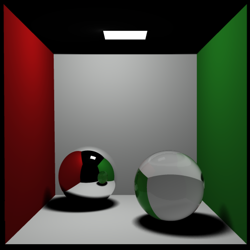
We started with the basic ray-tracer from Project 2. The first step was to create a scene file, and we decided to go for the Cornell Box. Since we were unable to find a .ray file for it, we looked at the description and created our own file. There was no support for area lights, and so we used a point light source, leading to the sharp shadows.
With the basic image done, we started with enhancements to the ray tracer. The first step was adding Fresnel reflection (at grazing angles, more light gets reflected than transmitted). We used Schlick's approximation since it was faster than the exact formula.

The next addition to the ray tracer was support for area lights. Area lights are implemented as a set of discrete point light sources whose positions are chosen using randomized stratified sampling. Adding distribution ray tracing along with the area lights gives us soft shadows.
With all the basic enhancements to the ray tracer complete, we started with photon mapping. Photon mapping is a 2-pass technique, and the basic idea is quite straightforward: each light source emits photons which get deposited on the scene. This is the first pass. In the second pass, we trace rays from the eye, and when we compute the intensity of a point, we add the contribution from the photon map.
Photons are emitted from the light sources in all directions. We use the photon map only for indirect illumination and caustics; the direct illumination is computed by standard ray tracing. When a photon intersects a diffuse surface, we store information about the power, position, and incoming direction. We use Russian Roulette to decide whether the photon is to be reflected, transmitted, or absorbed. The advantage of using Russian Roulette is that the number of photons traced doesn't increase exponentially with each bounce. Note that we only store photons which have bounced atleast once, because we are not interested in the direct illumination provided by the photons.
All the stored photons are then put into a balanced kd-tree. The advantage of using a kd-tree is that it allows for efficient queries to find the closest 'm' photons to a given point, with a worst case complexity of O(m.log(N)), where N is the total number of photons stored in the tree.
In the second pass, we trace rays from the eye towards the scene. When we calculate the intensity of a point, we also add the contribution from the photon map. To do this, we get the m closest photons from the point, and add their powers. This is then normalized by the area of the circle which contains these photons to get, the contribution to the intensity.
By considering only photons which pass through (or reflect off) specular surfaces, we can add caustics to the image.

Note that the scene file used in this image is slightly different. The area light is larger, and the camera position is closer to the screen (this gets rid of the box edges).
By considering all photons, we get the caustics and the global illumination. With this, the ceiling gets a bit brighter, and some light bounces off the walls onto the floor, adding some color to the otherwise dull floors.

Finally we rendered a few images of a transparent (floating) dragon in the Cornell Box.
Using a point light source, creating sharp shadows:
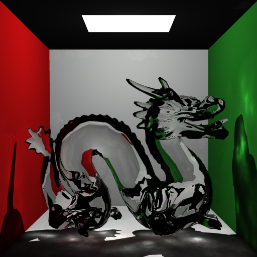
Same dragon rendered with lots of shadow rays (Rendering time 4.5 hours)

The floating blue dragon, with blue caustics.
