Methodology
To accomplish the experiment, we used the sample script on the webpage to create n eigenfaces and attempt recognition of the smiling faces given the eigenfaces (for each n between 1 and 33, inclusive, increasing by 2 each trial). The number of successful recognitions (out of 33) was manually counted and plotted.

In addition, we have here a file showing enlarged versions of the average face and the first 10 eigenfaces.

Finally, here are some examples of recognition errors that occurred in nearly every trial.

Questions and Discussion
1. The plot (observed above) shows a trend that is basically as expected: recognition is low for small numbers of eigenfaces, but increases rapidly as more eigenfaces are used. The accuracy appears to stabilize at 22/33 (67%) at around 5 to 7 eigenfaces, but may increase very slowly after that point. The tradeoff in deciding how many eigenfaces to use is thus one of accuracy versus performance. Although, since all eigenfaces are calculated at once, it takes the same amount of time (and space) to compute all eigenfaces, choosing a larger number of eigenfaces will cause later operations (namely, the ones, such as projection, which iterate over all eigenfaces) to take an amount of time that is roughly directly proportional to the number of eigenfaces used, the corresponding benefit being generally higher accuracy in the faces successfully recognized (and generally better MSEs for matches). Obviously, there is no clear answer to the question of how many eigenfaces to use; the answer is highly dependent on the face space itself (and the resultant map between eigenfaces used and accuracy), as well as how much accuracy and time cost is desired by the user. For this specific space, for instance, 5 eigenfaces would suffice for a reasonably accurate recognition, but more could be used if greater accuracy is desired.
Note 1. My accuracy was generally lower than the expected accuracy of 26/33 (79%); if there is some error in my code, it seems likely that it would be either a minor computational error in the recognition code or some minor notation error in the eigenface finder (e.g. accidentally shifting the eigenfaces or the input matrix by one row or one column). Any major computational error in either would dramatically change either the eigenfaces or the match results, as I observed when debugging.
Note 2. The fluctuation between 22 and 23 accurate matches between 5 and 11 eigenfaces is very interesting. It seems that it was due to a single incorrect matchup (smiling-23 to neutral-22) that was very close in MSE; adding different eigenfaces changed the MSEs by varying amounts, causing the fluctuation due to the overall closeness of the match. Face 23 was ultimately matched correctly, but not until several more faces were added (as observed in the plot).
2. Images of some common incorrect recognitions are shown above. As can be seen, all of the mistakes are actually fairly reasonable. The first match was likely made incorrectly because the smiling face photo was taken at a slightly higher altitude than the corresponding neutral photo, changing the relative position in the image of the mouth and nose. The second mismatch was likely made because the cropping caused the smiling face to be relatively larger than the corresponding neutral face, while the third was mainly due to the overall similarities between the incorrect and correct neutral faces. In fact, the incorrect and correct neutral faces are fairly similar in all cases; the correct matches, on further observation, were usually very high (second or third) on the list of closest matches because of this.
Methodology
First, taking the 10 eigenfaces and average face pictured above, used the face finder with the given parameters to crop elf.tga. The result:

(scale = 0.45 to 0.55, step = 0.01) No good. Perhaps color recognition would have helped my code to find actual faces, rather than simply taking the MSE, multiplying by distance from the mean, and dividing by the variance.
For the next step, we attempt to crop this picture of the professor.

(Image not to scale: scale = 0.12 to 0.16, step = 0.0025) Success! It's not the best crop, but, for a square image of the face, it's pretty decent.
Finally, we'll use two group photos. I'll use the third group of three students and the fourth class photo, and see how many faces the program can find.

(Image not to scale: scale = 0.8 to 1.0, step = 0.05, mark 3) Here we found two of the three faces and a nice section of wall. Sadly, no amount of fiddling with parameters could seem to get the program to recognize the third face. Again, color recognition might have helped; nevertheless, I'm not sure why dividing the score by the variance of the face didn't help get rid of the wall segments here (as wall segments can't be expected to have much overall variance)...

(Image resized 0.125x, also not to scale: scale = 1.0 to 1.3, step = 0.1, mark 20) Here we found four faces, somebody's shirt, and... 15 sections of wall. These are really poor results, but, as I'll describe later, I wasn't really able to improve the recognition much by tweaking the scoring system.
Questions and Discussion
1. All params given under each of the pictures above.
2. These trials were full of both false positives and false negatives. The most likely explanation for these seems to just be an overly simplistic scoring algorithm. While the MSE score seemed sufficient in most stand-alone cases to tell faces apart from non-faces, the fact that many thousands of faces are being tested could well produce anomalous cases where something different from a face would be scored higher than a face, causing both a false positive (as the other region was counted as a face) and a false negative (since the face itself was not). Most of the false positives seemed to be areas of wall; attempting to discourage the program from selecting these areas proved fairly problematic, since weighting the score too highly based on the variance would cause only the areas in the image with the most variance (e.g. sharp borders) to be considered, creating more errors since faces are not usually extremely high-variance regions. Hence, wall areas that (for some reason or another) match face space are a fairly common occurrence in these results. As I mentioned, color detection might have been a useful way to tell faces from walls or other areas, had I had time to implement it. Another potential factor besides the simplistic scoring algorithm that may have led to mismatches may have been the generally narrow range of scales that I had to use. As might be expected, the face-finding algorithm tended to take a very long time, especially on large images. In order to collect my results in a reasonable amount of time, then, I had to restrict the number of times that I cycled through the face-finding routine by reducing the range of image scales that I checked. Unfortunately, this may well have led to false negatives, as faces at scales that I did not check would, as expected, be far less likely to be considered as faces.
Methodology
First, we computed 6 25x25 eigenfaces for the neutral-faced students (identical to the first six of the ten eigenfaces above, of course) and then computed a userbase. Then we computed the set of MSEs for two sets of images: expected positives (each smiling image matched with the corresponding student) and expected negatives (each smiling image matched with the student with the preceding number, e.g. matching smiling-10 with neutral-9 and smiling-1 with neutral-31). Finally, we plotted the false positive count, the false negative count, and the total of the two for every threshold between 0 and 200,000 (incrementing by every 5,000). The results are below.
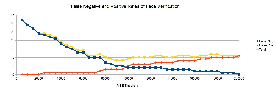
(Notice that, after 200,000, the total increases, since the false positive rate can only increase while the false negative rate is zero.) These results imply that the best threshold (namely, the one with the lowest total false match rate) is somewhere in the 90,000 to 95,000 MSE range. Finally, these MSE values may seem abnormally high (in some cases, expected negatives produced MSEs of over 1,000,000); this is due to the small number of eigenfaces, which, as observed before, tends to produce worse matches in general.
Questions and Discussion
1. Technically, I did not try any MSE thresholds, since I used an alternate method to find the optimal threshold. I took the expected positive and expected negative cases and simply computed the MSE for each match. This makes it trivial to find the false positive and false negative rates given any threshold; for each expected positive MSE, if the threshold is less than that value, the expected positive is declared a negative, resulting in a false negative. Similarly, for each expected negative MSE, if the threshold is greater than that value, the expected negative is declared a positive, resulting in a false positive. This, of course, makes finding the optimal threshold quite easy, as a costly and time-expensive search is not required. (Note that I plotted the rates for every threshold between 5,000 and 200,000, inclusive, with a step rate of 5,000.)
2. The best threshold (between 90,000 or 95,000, given these samples) produced a false positive rate of 3/33 (9.09%) and a false negative rate of 5/33 (15.15%), for a total mismatch rate of 8/66 (12.12%).
Just the morphing. It was easy, and it seems to work well.