(Note: 'we' in the below is used in the proverbial sense, and all work was performed by the above student.)
In
this project, we used PCA to perform face detection in images. The
process involves constructing a vector subspace in the space of images
such that faces are well represented by linear combinations of the
subspace basis vectors. The first step is to input a number of training
samples into the algorithm, find the average face, and then compute the
delta from the average face to each sample face. These deltas are then
used to contruct a covariance matrix for each sample image, and
these matrices are summed into an overall covariance matrix A. By
finding the largest n
eigenvectors of A, which represent the variance of the faces in various
directions from most variant to least, we then construct a basis set
that represents the images with an arbitrary degree of accuracy (if all
of the eigenvectors are used then we can perfectly reconstruct the
training set). A new image can then be projected into this space by
first subtracting the average face and then taking the dot product of
the residual with each basis vector, yielding a set of coefficients
which can be used to construct the closest image on the hyperplane to
the new image.
We can then perform various feats with this
reconstruction. We can, for example, represent each training sample by
its coefficients and then given a new image we can take its projection
and determine the distance to each training sample in face-space,
taking the closest such sample as the "recognized" sample (not unlike a
nearest neghbor classifier). Another interesting application is
face detection. In this application we take an input image and move a
window over it at various locations and scales. For each subimage so
defined we can compute its projection in face-space and then
"reconstruct" the original image using only a linear combination of the
basis vectors. Then we can take the difference between the original and
the reconstruction and apply a threshold to decide if it is a face or
not. The approach is a bit naive and the accuracy is not terribly good
without some additional heuristics (some of which we tried and will
discuss below). The overall concept is quite a useful one and is common
in statistics, computer vision, and machine learning fields. It was
challenging to implement and fun to apply it in a doiman where we get
to see what eigenvectors look like.
The
most challenging part of the project was definitely face detection. The
basic algorithm of thresholding distance to the hyperplane ended up
detecting lots of garbage. Many additional heuristics were applied in
an attempt to improve the accuracy of this part of the project, and the
best performing such heuristics were left in the final code. Hopefully
it performs well on test data but its clear that building a robust face
detector on top of PCA would require quite a bit of time, lots of
training data, and plenty of creativity. Other algorithmic aspects of
this problem were also challenging, including ensuring that overlapping
windows were not returned in the result set, and generally keeping
track of the various coordinates and scales involved.
As
a result of this project we learned a technique for constructing a
linear subspace from samples in a vector space. This approach can
be used for recognition of previously seen samples and for recognition
of new samples, for compression and dimensionality reduction, for
feature selection, and for a variety of other applications. It was
quite interesting and fun to try it out in the context of face
detection as this gave us an opportunity to literally see the results
of the process. It was also interesting to see how it worked in
practice on unseen data and fun to explore various heuristics to
improve its classification performance.
The
project involved filling in major functionality in the skeleton of a
face recognition program. The program was written using Microsoft
Visual C++ and came with a number of important routines already
written, including support for reading and writing images, vector
operations, image manipulation, and some important mathematical support
routines such as the Jacobian algorithm for computing
eigensystems.
The follow describes the routines implemented:
- Faces::eigenFaces
- This routine computes the average face and the set of "eigenfaces".
The latter are the eigenvectors associated with the largest eigenvalues
for the matrix composed of the sum of the covariance matrices for the
residuals of the training faces after removing the average face. These
vectors form a basis for "face space" which is used in the various
other routines.
- EigFaces::projectFace - This
routine takes an image and projects it into "face space". First the
average is subtracted from the input vector and then the vector is
projected onto each eigenvector, producing a set of coefficients
representing the coordinates of the residual in eigenspace.
- EigFaces::isFace
- This routine projects a face into face space and then computes the
mean squared error of the difference in pixels between the
reconstructed projection and the original. This routine is
important for the findFace routine below.
- EigFaces::verifyFace - This routine compares the projection
of an input face into face space with the coefficients of another face
in face space. The mean squared error of coefficients is used to
determine closeness of the input face to the comparison face on the
face hyperplane. This routine is used for recognizeFace below.
- EigFaces::recognizeFace - This routine takes an input face and uses a precomputed database of coefficients
for known faces and runs them through verifyFace. The MSE for each is
computed and the known face with the lowest MSE is returned to the
caller. It is used to classify a new data point as one of the
previously known data points in a nearest-neghbor fashion.
- EigFaces::findFace - Definitely the most challenging part
of the assignment, this routines job is to search an image for faces.
The routine steps through a number of scales at a given increment,
scaling the input image to each. It then walks the image field with a
window of a fixed size (in scaled space). Each such window is tested to
see if it is a face. Initially this was implemented with a simple call
to isFace but this proved to be... non-robust. Additional processing
was added to this method including multplying the MSE by the distance
of the input image to the mean face, and dividing by the pixel variance
of the input image. This penalized windows which were far from the
average face in pixel space, and rewarded windows which had complex
texture in them. This still proved not sufficient for recognizing the
baby in the elf test image so skin color queues were added to the
routine. The average color of skin was computed directly from the
baby's face and a heuristic was designed to penalize windows whose
average color was far from this. Later experiments were done using
multiple skin tones but any change to the skin tone heuristic seemed to
ruin detection of the babies face, even though it may have improved
detection of other faces. In the end the simple baby-face heuristic was
left in place to ensure that cropping worked with the parameters
specified in the assignment. An idea for future research is to use PCA
to form a vector subspace of skin colors, and use an approach similar
to the way we classify faces here to classify the color of an image
window. More time was needed to see if this would really work in
practice. I suspect that a simple average is not sufficiently
descriptive to be very helpful. A space of histograms would probably
yield the best results.
In
this experiment we constructed an eigenspace using the non-smiling
students dataset, which consisted of cropped pictures of students from
our class in "neutral" expressions. We used the entire set of pictures
to create a set of 10 eigenvectors of size 25x25 pixels to represent
the subspace. The average face and the 10 eigenvectors are shown below:

Average face using the non-smiling student pictures
The 10 eigenfaces produced from our class non-smiling dataset, 0-4 on the top row, 5-9 on the bottom row.
With these
eigenvectors in hand we then computed a "userbase" consisting of the
coefficients for each of our input samples in eigenspace and then
attempted to classify each of the original persons. Instead of using
the original images however, we now used the "smiling" images. These
pictures had our students in various facial poses, in an attempt to
make things more difficult for our recognition program. To give the
reader an idea of how difficult, here is a sample from the "smiling"
collection.

In
order to get a sense of how the algorithm performed, we swept the
number of eigenfaces used from 1 to 33, in steps of 2, and computed the
number of correctly recognized faces. The results are given in the
chart below. Apologies for the scaling on the chart, we
could not get Kompozer to scale the image any large in the y direction.
Click on it to see the full size image.
Questions
1.
Describe the trends you see in your plots. Discuss the tradeoffs; how
many eigenfaces should one use? Is there a clear answer?
It
appears that there is a sharp increase in accuracy initially, then a
period of gradual improvement seasoned with periodic reductions in
accuracy. It is expected that the accuracy improve quickly, since the
eigenvectors are order by their contribution to the overall variance in
the images seen. As we increase the number of eigenvectors used, we are
going to have less interesting eigenvectors to choose from. The
undulation in the accuracy is probably because the set of eigenvectors
with largest eigenvalues does not capture certain subtleties in the
data, and sometimes the eigenvectors with smaller eigenvalues are
needed in the basis set in order to correct innacuracies introduced by
the larger ones. One interestng point is that we might have expected to
see 100% accuracy with 33 eigenvectors, since the entire space could be
spanned, but this is not the case since these are completely new
images. In fact we did try this on the original input images and 100%
accuracy was achieved well before 33 eigenvectors.
2.
You likely saw some recognition errors in step 3; show images of a
couple. How reasonable were the mistakes? Did the correct answer at
least appear highly in the sorted results?
We did see plenty of recognition errors, as explained above. Here is an example:

The input image. | 
The first guess. | 
The second guess. | 
The third guess. |
While
it seems clear for a human observer that these first three images
are not the same people (humans are incredibly sensitive to queues used
for identifying other humans) it may be reasonable for the computer to
make these mistakes. The skin tone, highlights, and shadows in
these images are similar, and the fact that the person on the left
is sticking his tongue out makes it look similar to the mouth of the
person on the right. The noses and eyes are clearly different, even at
this low resolution, but we can see how the algorithm might have made
this mistake. The actual person we were looking for was in fact third
in the list of images selected by the algorithm as matches for this
input image. Based on the metic we used we can see why this might be
the case. The last image has a much thinner mouth area, lighter creases
around the mouth, and a darker overall skin tone.
In
this experiment we used the same of eigenvectors we used in the
previous experiment to automatically detect unknown faces in
various images.
In the first part of this experiment we used the program to crop a face from a given image (the "elf" image)
automatically. The scale parameters were swept from .45 to .55 at
increments of .01. The source image and the final cropped image are
shown below.
 |  |
The original "elf" image (showing detection box) and the cropped version using our face detection algorithm.
This
took quite a bit of tweaking to get right. Initially we used just the
basic detection algorithm (distance of the reconstructed image on the
face hyperplane to the original image) but this proved to be woefully
innacurate. We were getting boxes in all sorts of places except for
faces. The algorithm tended to like the top left corner of the bald
mans head for some reason. Frequently the windows that came back, even when a number of them were used such as 10, included no faces at all. This
was quite frustrating as we scoured our code for bugs. We could not
find any. So we set about attempting to improve the algorithm
heuristically.
The
first thing we did was to implement the
suggested hack in the project write-up. Unfortunately the description
of this hack could have been intepreted as using distance and variance
in face-space or in pixel-space. Since we were frequently seeing boxes
on the walls (low variance in pixel space) we elected to implement the
scheme using pixel
coordinates. So we penalized the distance of the window image from
the average face and rewarded windows images with high variance. This
resulted in no more walls and our baby's face was now in the top three
faces detected but it was not the top face. The top face was a box
including the bald mans right shoulder and the babies hand. So in
desparation we elected to try color queues. We took the babies face,
cropped it, and computed the average color. This was used in our code
to provide a distance metric in color space and by incorporating this
into our face score we were finally able to get the babies face to crop
correctly.
Another interesting point about this picture was that
the bald man was never recognized, not even once, with all the
varieties of settings and heuristics we tried. It must be the case that
his face is too far from the face hyperplane, probably due to his
glasses, bald head, and the cocked orientation of the face with respect
to the image axes.
1. What min_scale, max_scale, and scale step did you use for each image?Each
image required a different seting for these parameters., which was
determined by manual exploration and looking at the size of the
detected "faces". For the "elf" image, we used the settings prescribed
by the assignment and then did tweaking of the algorithm in order to
get the crop to work correctly. The other images were played with until
the boxes were roughly correct and then a range was specified around
that point. The step size was set to give a nice sweep, say ten or so
scalings per image
2. Did your
attempt to find faces result in any false positives and/or false
negatives? Discuss each mistake, and why you think they might have
occurred.
See the detailed analysis of results below.
eigenfaces --findface me.tga eigenfaces.txt .06 .1 .001 mark 4 me_faces.tga
This
is a large image, .originally 1003x1172 pixels. Despite dramatic
scaling and sweeping a large range of parameters we were unable to get
the only face to be detected. Instead the program selected an area
consisting mostly of wall texture. This may be a confusing image for
our face detector since there is a lot of featureless wall in the
image, and the wall is roughly skin-toned. The high resolution may
cause the image to darken significantly when it is scaled down or may
cause aliasing or other artifacts to occur that might inhibit the
detection process. Since our algorithm includes a heuristic to detect
face colors, the wall color here may be getting extra points that cause
the algorithm to misdetect it as a face.
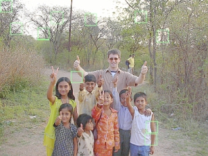
eigenfaces --findface india.tga eigenfaces.txt 1.0 1.2 .1 mark 10 india_faces.tga
This
was a smaller image, 400x300 in size. Unfortunately the algorithm
seemed very distracted by all the trees in the background and did not
detect any faces. Its possible that the heuristics added for variance
maybe have caused the algorithm to favor the highly variant areas with
trees and sky. Other areas that seemed to get preference included the
drab section of road highlighted. My face in this picture includes
sunglasses which may have confused the algorithm further.
eigenfaces --findface "..\faceimages\group\group_neutral (2).tga" eigenfaces.txt .3 .6 .1 mark 3 group_neutral(2)_faces.tga
This
was a medium sized image 600x400 in size. We had the program sweep the
scaling from .3 to .6 in increments of .1 and mark the top three faces.
We were delighted to see that we got two out of three faces correct.
The program apparently thought that the guy on the left's elbow was
more face-like than the guy on the right's face. We were not entirely
sure why this would be. Our face detector uses reconstruction error,
distance from the average face in pixel space, penalizes low-variance
windows, and prefers skin tone. The reconstruction error and distance
from the average face seem like they should favor the face on the
right. The elbow window seems like it should have lower variance in
pixel space and so it should be penalized. The skin tone component
should be about the same on both, although perhaps this is the culprit
since the face on the right has more dark tones in it. Perhaps a more
sophisticated skin tone detector would help with this image.
 |
 |
eigenfaces --findface ..\faceimages\group\class_pano_handheld.tga eigenfaces.txt .1 .7 .01 mark 33 pano.tga
This
was a very large image with loads of faces and lots of artifacts due to
the panorama stiching process. The viewer can click on the lower image
to get a full resolution version - its easier to see the boxes in the
full resolution image. This image produced a high number of false
positives but did manage to find three faces. Looking at the various
patches detected as faces I would say that there seems to be too much
preference for high variance in our algorithm and not enough emphasis
on the closeness to average face. I think that training on a much
larger dataset, using more eigenfaces, and preprocessing each subimage
for contrast invariance might be helpful.
In
this experiment we used the -verifyface feature of our executable to
determine if a picture was of a particular individual. First we created
an eigensystem with 6 eigenfaces using the "non-smiling" class training
dataset. Then we ran a test for each individual using a known positive
picture (the individuals corresponding "smiling" photo) and a known
negative picture (a randomly selected "smiling" photo of a different
individual). We then swept the MaxMSE parameter for the verify face
function from 0 to 1150000 in increments of 10000 (we determined the
range with an initial low resolution sweep - a finer step might
have resulted in a prettier graph but would have taken longer to run)
and recorded
the true positive and false positive rates for each setting. With this data in hand we create an ROC plot so we could examine the performance visually.
1. What MSE thresholds did you try? Which one worked best? What search method did you use to find it?
The
MSE's used were 0 to 1150000 in steps of 10000. We did an initial lower
resolution parameter sweep to determine the range of interesting
values. This range of values encompassed all behaviors including
getting all the positive right, all the positives wrong, all the
negatives right, and all the negatives wrong.We might have used a finer
step size for producing our data but we are short on time here.
2. Using the best MSE threshold, what was the false negative rate? What was the false positive rate?

Using
the ROC plot we can choose the point which maximizes the criteria we
are interested in. For example, if our primary goal is to recognize
known individuals as often as possible and we dont mind a few false
positives, we might choose the point at 0.27 false positive rate, and
1.0 true positive rate (i.e 0 false negative rate) (which corresponds
to
a threshold of 200000) which gets all of our positive examples correct
but thinks that 27% of our negative examples are positive examples. On
the other hand suppose we were using this to build a security system
and so
false positives were very, very bad. Then we might choose the point
which minimizes false positives first, and maximizes true positives
second. That point is at 0 false positive rate, and 0.46 true positive
rate (i.e. 0.54 false negative rate) and corresponding to an MSE
threshold
of 40000. So I would say that the "best" MSE really depends on your
application. Apologies for the scaling on the chart, we could not
get Kompozer to scale the image any large in the y direction. Click on
it to see the full size image.
We
attempted to improve the performance of the face recognition classifier
by adding a skin tone component. To do this we took the "elf" picture,
cropped the babie's face and then took a histogram which gave us
average red, green, and blue values. We encoded that into a reference
vector in our findFace function and then for each window under
consideration we computed the average color in the window and penalized
the window by the distance of this average color from the skin tone. We
experimented with support for multiple skin tones, and even started to
implement a PCA version of this but time ran out and we reverted to the
simple baby skin tone detector in order to ensure that we were able to
automatically crop the baby (for some reason it really liked the man's
elbow, hmmm... it likes elbows in general). Our PCA idea is the take a
variety of average skin tone vectors and consider these to be
"examples" of a linear color subspace, just like we consider faces to
be examples in a linear subspace of pixels. We would then construct the
average skin color, the matrix A of convariances of skin color
residuals, and compute the eigenvectors of our skintone subspace. This
would allow us to perform a procedure not unlike the face detection
procedure, that would help us to more accurately determine if a window
was a skin area. It would probably be a good idea to use a histogram
instead an RGB vector for this since that would capture more
information about the distribution of colors. Given more time I think
this would be a really cool thing to try.