CSE576 Project 1
Feature Detection and Matching
Aditya Sankar (aditya at cs)
April 16, 2013
Feature Detection
Points of interest, or corner points were detected using the Harris corner detection. The Harris score for each point was calculated with the following algorithm (adapted from [1]):
1. Convert image to grayscale
2. Compute horizontal and vertical gradient images Ix and Iy by convolving gray image with Sobel kernels in the X and Y directions.
3. Compute outer products Ix^2, Iy^2 and IxIy
4. Convolve each of the three images with a 7x7 Gaussian
5. Compute corner strength with formula R = det(M) - k(trace(M))^2, with k=0.05
6. At this stage also store the dominant direction of the interest point by smooting X & Y gradients in a 7x7 window and calculating angle as arctan(gradY/gradX)
7. Finally, interest points are those that are above a threshold (0.1) and are local maxima in a 3x3 window
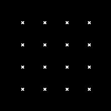
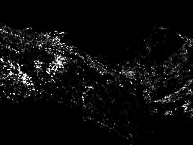
Fig 1. Checkerboard pattern (a) and its Harris response (b). (c) shows detected feature points in red.
Feature Description
Two separate feature descriptors were implemented to describe each feature point:
Simple 5x5 Window: A 5x5 square window around the point of interest is selected and the pixel values are serialized into a feature vector of size 25.
MOPS (simplified): A simplified version of the MOPS descriptor[2] was implemented. A 39x39 window is selected around the point of interest. The window is pre-rotated by the dominant gradient at that point (calculated above, in step 6 of the Feature Dectection process). The rotation is achieved by inversely mapping image pixels into rotated window pixels. Bilinear interpolation of values was used for points that lie between two pixels. If the rotated window falls outside the original image, the feature is discarded. Once the window patch has been extracted, it is prefiltered with a gaussian and sampled into an 8x8 patch by extracting every 5th pixel. The 8x8 patch is then serialized into a vector of length 64. The brightness values are normalized normalized by dividing by the square root of the sum of the squares. The algorithm is summarized as follows:
1. Select a 39x39 window around point of interest
2. Rotate the window according to dominant gradient at the interest point
3. Read in the pixel values by inversely mapping from the image (with bilinear filtering)
4. Prefilter with a 7x7 Gaussian kernel
5. Subsample to get an 8x8 patch
6. Normalize intensities in the 8x8 patch
7. Serialize pixel values and store as feature descriptor
Feature Matching
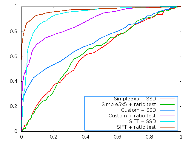
A ratio test was implemented that calculates the ratio of the best match score to the second best match score. This resolves ambiguous matches and avoids spurious matches when there is repeated structure or texture. The ratio test on average performs better than the simple sum of squared differences (SSD) approach, as can be seen from the performance analysis section.
Design Choices
Harris corner detection was efficient to implement as it does not involve the computation of a square root. Also precomputing dominant patch gradient at this point seemed efficient. All convolutions assume a repeating border. This reduces the corner response at edges, which is generally OK for most matching applications.
The Simple 5x5 descriptor is only invariant to position. In contrast, the MOPS descriptor is invariant to position, orientation (due to the rotated window) and illumination (due to the intensity normalization). Bilinear interpolation was used to calculate pixel intensities of the rotated patch providing sub-pixel accuracy. The multi-scale aspect of MOPS was implemented for extra credit by running the above detection and description algorithms on 4 levels of the gaussian image pyramid. The resulting features were scaled back to map to the original image. I did not implement the haar wavelet analysis mentioned in the MOPS paper and leave that for future work.
A lot of time was spent in debugging the image library provided. Off-by-one errors and image shifts were causing issues in the project. I hence decided to implement my own patch rotation and interpolation code. Modifications were made to the library's convolution code as well.
Performance Analysis
Harris Reponse (scaled)
| yosemite |
graf |
|  |
ROC Curves
| yosemite |
graf |

|  |
Benchmarking Results
Simple 5x5 Window Descriptor
|
SSD |
Ratio |
|
Average Error |
Average AUC |
Average Error |
Average AUC |
| graf |
282.38 |
0.542 |
282.38 |
0.577 |
| wall |
346.56 |
0.490 |
346.56 |
0.618 |
| leuven |
401.55 |
0.309 |
401.55 |
0.502 |
| bikes |
331.32 |
0.698 |
331.32 |
0.764 |
Custom MOPS-based descriptor
|
SSD |
Ratio |
|
Average Error |
Average AUC |
Average Error |
Average AUC |
| graf |
242.55 |
0.587 |
242.55 |
0.684 |
| wall |
267.27 |
0.681 |
267.27 |
0.847 |
| leuven |
315.18 |
0.736 |
315.18 |
0.761 |
| bikes |
293.78 |
0.699 |
293.78 |
0.908 |
Strengths and Weaknesses
The custom descriptor is designed to work well with chances in translation, rotation, scale and illumination. The benchmark datasets provide variations in these attributes. In particular the leuven datasets offers large changes in illumination, resulting in slightly lower performance. The graf dataset has translation, rotation and scale and is the most difficult to match, as indicated by the AUC score.
Detecting features at multiple scales helps with the bikes and wall dataset, where a significant improvement is noted. The descriptor also performs well on 3D rotations. Further improvement may be achieved by implementing a gradient histogram based approach, such as SIFT.
Overall, the custom descriptor seems to do a good job on the datasets, but lags behind SIFT, which is the state of the art.
My Test Images
I took two pictures of the Suzallo Library on the UW campus. As an added challenge there is a large variation in 3D rotation, scale (zoom) and the facade has a lot of repeated structure. However, it seems like the feature matching works fairly well (green features match).
 |
| Test results. Click image for larger view. |
Extra Credit
Adaptive non-maximum suppression (ANMS)[2] was implemented in order to provide an even spread of features. The features selected via ANMS are not necessarily the strongest, but are the most spatially dominant in their region. Much in the same way that Mount Rainier is the most 'topographically prominent' mountain in the contiguous United States, but not the tallest. A wider spread of features can lead to more efficient matching for large datasets, but in general degreades the ROC curve of the descriptor (eg. decrease from 0.934899 to 0.903805 in Yosemite dataset). Hence ANMS was not enabled in the benchmarks. Some visual results are shown below. Click images to expand.
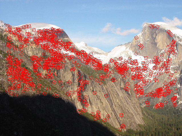
|  |
| Without ANMS | With ANMS (500 most dominant features) |
Multi Scale Descriptor:
Implemented feature detection at multiple scales using Gaussian pyramid approach as described above. This makes the descriptor invariant to scale and improves performance on graf and wall dataset that show large changes in scale/zoom.
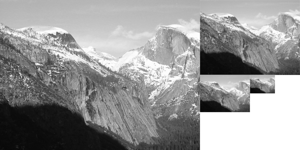 |
| Gaussian Image Pyramid for the Yosemite image. |
Configuration Notes
- Operating System: Linux 64 bit, Fedora 17
- Changes to arguments: [featureType] 1-simple5x5 (Default), 2-Custom Descriptor
- Changes to framework: Bug fixes in Convolution, Warping
References
[1] Szeliski, R., Computer Vision: Algorithms and Applications, http://szeliski.org/Book/
[2] Brown, M., Szeliski, R., and Winder. Multi-Image Matching Using Multi-Scale Oriented Patches.
--