Contents

Feature Detection
Feature Descriptor
Feature Matching
Performance
Discussion
Extra Credit
References

CSE 576 Project 1:
Feature Detection and Matching

Haoming Chen
eehmchen at u dot washington dot edu
April 18, 2013

Feature Detection

Multi-Scale Pyramid[1] (Extra Credit)

To make the feature more invariant to scale, a pyramid of images with different scales can be utilized. In this project, I create this pyramid of images of 5 levels as follows:

Filter the low level image (level l) with a Gaussian kernel ([1 4 6 4 1]/16 in separable two dimensions).
Downsample the blurred image and save it as the up level image (level l+1).
Repeat process 1 and 2 until get a 5 level (level 0-4) of pyramid.

For each image in different level of the pyramid, we do the same operations (corner detection, ANMS, decription and so on), which are discussed in following parts.

Harris Corners

Given a image at level l, the first step is to find interest points in the image. For every point in the image. A Harris matrix can be generated as follow [1]:

H_l(x,y) = \nabla_{\sigma_d}P_l(x,y) \nabla_{\sigma_d}P_l(x,y)^T * g_{\sigma_d}(x,y)

The "corner" strength function is

f_{HM}(x,y) = \frac{\text{det} H_l(x,y)}{\text{tr} H_l(x,y)} = \frac{\lambda_1\lambda_2}{\lambda_1+\lambda_2}

Followings are Harris image for Yosemite and graf:

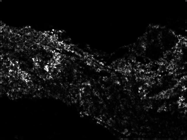Harris Image of Yosemite

Harris Image of graf

Adaptive Non-Maximal Suppression[1] (Extra Credit)

After calculating the Harris value, what we want are the points with the largest value, which means it is more likely to be a corner. One method is to set a threshold and select the points with value larger than it. However, it is not easy to choose a proper threshold adaptively and the selected points may have many overlap. Instead of setting a threshold for the whole image, the Adaptive Non-Maximal Suppression algorithm can select the interest points with better spatial distribution.

The main idea of this method is to select the point which is maximum over a large area. A minimum suppression radius $r_i$ calculated to measure the area, as:

r_i = \min_j |x_i - x_j|, \text{ s.t. } f(x_i) \le cf(x_j), x_j \in \mathcal{I}

where $x_i$ is a 2D interest point image location and $\mathcal{I}$ is the set of all interest point locations. The value $c = 0.9$ is to ensure that neighbor must have significantly higher strength. In this project, we select the 500 interest points with largest values of $r_i$

The following figures compare the results of using regular detection (local maximum in the $3\times 3$ window and above a threshold) to the AMNS. It is obvious that features are distributed better across the whole image.

Regular detection (maximum in local 3×3 window)

Adaptive Non-Maximal Suppression

[back to top]

Feature Descriptor

Rotation Invariant (Extra Credit)

Similar as discussed in the lecture sides, an orientation anlge θ=atan(dy⁄dx) could be derived. After getting the angle, I rotation the 40×40 window to the horizontal direction. After rotation, an 8×8 image patch is sampled with a stepsize of 5 in the 40×40 window. We use this 64 values as the descriptor vector

Contrast Invariant (Extra Credit)

After sampling, the descriptor vector should be normalized to make the features invariant to intensity. Finally, the feature vector will have zero mean and one standard deviation.

[back to top]

Feature Matching

Two matching methods are evaluated in this project: sum of square difference (SSD) distance and ratio score. SSD is the summation of square differences between elements of the two descriptors. I implemented the other method called ratio test. The ratio score is the ratio of the best match SSD and the second best match SSD. A smaller ratio score means a better feature point.

[back to top]

Performance

ROC curves for Yosemite and graf

ROC curves for Yosemite

ROC curves for graf

Average AUC on 4 Benchmark Sets

SSD match

	average error	average AUC
bikes	245.904784	0.635211
graf	289.679639	0.568391
leuven	262.119331	0.649965
wall	254.218998	0.533478

Average AUC on 4 Benchmark Sets (SSD match)

Ratio Match

	average error	average AUC
bikes	245.904784	0.899729
graf	289.679639	0.680809
leuven	262.119331	0.861150
wall	254.218998	0.746586

Average AUC on 4 Benchmark Sets (ratio match)

I also evaluate different scenarioes those are w/ and w/o the pyramid structure and ANMS to see whether they improve the performance.

Without Pyramid (extract 2000 points in original level, ratio match)

	average error	average AUC
bikes	304.108791	0.849347
graf	303.153780	0.698413
leuven	283.916442	0.836846
wall	315.313407	0.818150

Average AUC on 4 Benchmark Sets (w/o pyramid, ratio match)

We can see the the error increase for all 4 dataset and the for "bikes" and "leuven" the average AUC also drops.

Without AMNS (only 3×3 local maximum Harris value, ratio match)

	average error	average AUC
bikes	183.982601	0.889333
graf	239.170204	0.650636
leuven	264.051454	0.874434
wall	231.801160	0.739099

Average AUC on 4 Benchmark Sets (w/o pyramid, ratio match)

[back to top]

Discussion

According the experiments, we can see that the pyramid structure is efficient and the ANMS algorithm can work well. For the bikes dataset, some images are blurred, so the pyramid can improve much better. I found that with and without ANMS, the performace didn't change too much.
However there are more work can do. When doing rotation, I just use the nearest neigbour. A interpolation can be used to improve the accuracy.
[back to top]

Extra Credit

All the refined implementations are from MOSP paper.

Bulit a Gaussian image pyramid and extract features from each level, scale invariant. (explained earlier)
Implement adaptive non-maximum suppression. (explained earlier)
Normalized the feature vector to make it contrast invariant. (explained earlier)
Computer the orientation angle and rotate the feature to make it rotation invariant (explained earlier)

[back to top]