Feature descriptor
I used a single-scale variant of MOPS for a feature descriptor. For each detected feature, the algorithm applies the following operations to generate a descriptor:
- Compute the angle of the pixel based on the convolution of 9x9 horizontal and vertical Sobel filters with the grayscale version of the image.
- Acquire a 40x40 subimage of the grayscale image centered at the pixel after it has been blurred using a 7x7 pixel Gaussian filter with σ=2.0, then compute the mean and standard deviation of its values.
- Rotate the 40x40 subimage toward "up" relative to the computed angle of the pixel.
- Sample 18 values from concentric circles of radius 5, 10, and 20 about the pixel from the subimage. This technique was proposed in a student's project from a previous quarter and produces better data for the descriptor than simply using a grid.
- Subtract the mean from each sampled value and then divide by the standard deviation to account for differences in illumination.
Design choices
I chose to implement a variant of MOPS simply out of curiosity. The rest of the techniques fell into place through reading and experimentation; I found that using larger Sobel filters and the Gaussian kernel led to better scores in the benchmarks.
Performance
ROC curves
Here are the ROC curves for the graf and yosemite image sets provided with the project. The Harris threshold was set to 10 (on a semi-arbitrary scale) to generate the curves.

The area under the curve (AUC) for the graf image set is a low 0.47568 when using MOPS plus the SSD test, but is much higher, at 0.981271, when using MOPS plus the ratio test.
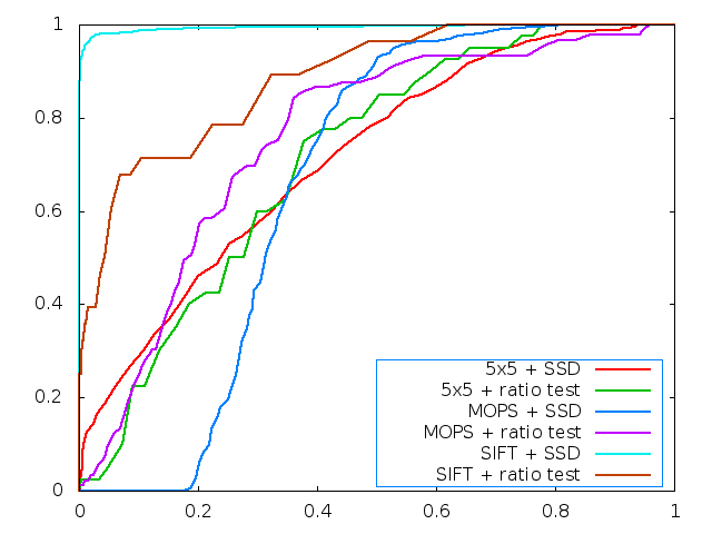
The AUCs for the yosemite image set are 0.662229 when using MOPS plus the SSD test and 0.756059 when using MOPS plus the ratio test.
Harris operators
Here are the Harris operator images produced by running feature detection on the graf and yosemite images.
graf Harris operator image

yosemite Harris operator image

Average AUC for benchmark sets
The following is a report of the performance of the feature detection and matching on four different benchmark sets.
| Benchmark name | bikes | graf | leuven | wall |
|---|---|---|---|---|
| img1 AUC | 0.457351 | 0.545338 | 0.072379 | 0.172003 |
| img2 AUC | 0.439248 | 0.475632 | 0.008186 | 0.187861 |
| img3 AUC | 0.420252 | 0.77915 | 0 | 0.174284 |
| img4 AUC | 0.352668 | 0.544325 | 0 | 0.460291 |
| img5 AUC | 0.341132 | 0.338019 | 0 | 0.260319 |
| Mean AUC | 0.4021302 | 0.5364928 | 0.016113 | 0.2509516 |
| Median AUC | 0.420252 | 0.544325 | 0 | 0.187861 |
| Benchmark name | bikes | graf | leuven | wall |
|---|---|---|---|---|
| img1 AUC | 0.503754 | 0.607881 | 0.174869 | 0.211139 |
| img2 AUC | 0.506199 | 0.552674 | 0.042857 | 0.249494 |
| img3 AUC | 0.537099 | 0.597185 | 0 | 0.172718 |
| img4 AUC | 0.435306 | 0.484037 | 0 | 0.225602 |
| img5 AUC | 0.414593 | 0.099666 | 0 | 0.235734 |
| Mean AUC | 0.4793902 | 0.4682886 | 0.0435452 | 0.2189374 |
| Median AUC | 0.503754 | 0.552674 | 0 | 0.225602 |
| Benchmark name | bikes | graf | leuven | wall* |
|---|---|---|---|---|
| img1 AUC | 0.775454 | 0.47568 | 0.552104 | 0.685016 |
| img2 AUC | 0.784334 | 0 | 0.60273 | 0.658239 |
| img3 AUC | 0.797402 | 0.426372 | 0.628107 | 0.604564 |
| img4 AUC | 0.774967 | 0.131104 | 0.632951 | 0 |
| img5 AUC | 0.793431 | 0 | 0.628162 | 0.329022 |
| Mean AUC | 0.7851176 | 0.2066312 | 0.6088108 | 0.4553682 |
| Median AUC | 0.784334 | 0.131104 | 0.628107 | 0.604564 |
| Benchmark name | bikes | graf | leuven | wall* |
|---|---|---|---|---|
| img1 AUC | 0.71926 | 0.982255 | 0.710841 | 0.722628 |
| img2 AUC | 0.70888 | 0.50659 | 0.693035 | 0.710747 |
| img3 AUC | 0.679203 | 0.809851 | 0.603455 | 0.626793 |
| img4 AUC | 0.667751 | 0.740979 | 0.615342 | 0.886966 |
| img5 AUC | 0.766179 | 0.811105 | 0.649444 | 0 |
| Mean AUC | 0.7082546 | 0.770156 | 0.6544234 | 0.5894268 |
| Median AUC | 0.70888 | 0.809851 | 0.649444 | 0.710747 |
*I used a Harris threshold of 0 for the benchmark using the wall image set. Some images still resulted in AUC scores of 0, but the scores for the others were significantly better than they were at a threshold of 10.
Strengths and weaknesses
My descriptor is missing the "M" part of MOPS and hence does not perform as well as it could across affine and scale transformations. In comparing the first image to the last image of the wall image set, for instance, the bricks differ significantly in apparent size due to the affine transformation caused by imaging the wall from an angle as opposed to head-on. Even with a large number of descriptors from setting the Harris threshold to a low value of 0, the match algorithm fails to find any true correspondences between features using the ratio test. Overcoming this limitation would be a matter of sampling images at multiple scales to generate the feature descriptor in line with the original idea of MOPS.
The descriptor performs reasonably well for translations and rotations, however, as evidenced by the respectable scores for the other benchmark sets; in particular, the graf image set showcases the ability of the descriptor to work well with rotations using the ratio test, such as between the first and second images where the AUC is 0.98. What is interesting is how poorly the descriptor performs using simple SSD, however, where the graf scores are abysmally low. I theorize that the ratio test does better at identifying meaningful descriptors between images, whereas there are likely many false positives when using only SSD. Using a large (40x40) downsampled image patch in generating the descriptor helps performance on the bikes image set, where a Gaussian blur has been applied to an input image. Subtracting the mean of the image patch and then dividing by the standard deviation also helps to account for differences in lighting between images as well.
Real-world performance
To test the real-world performance of my system, I used an image of a hummingbird that I had taken with the camera on my smartphone. The focus is not that good in the image and there is some distortion due to movement, since I was trying to take a picture quickly.

For input images, I used a simple cropped subset of the image around the hummingbird and feeder as well as a rotated, brightened image. The red lines in the image below indicate which feature points the system determined were in correspondence with which other feature points.
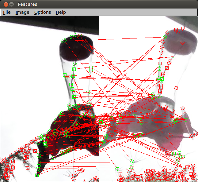
There are quite a few false positives, but the system does a reasonably good job of matching feature points related to the "stem" at the center of the glass receptacle as well as some of the "flowers" around the base.
Extra credit
My feature descriptor did not perform as well as I would have liked, but it is theoretically robust to translations, rotations, and changes in illumination and gives some indication that it is.