Computer Vision
CSE 576 Spring 2013
Project 1: Feature Detection and Matching
Kevin Huang
Feature Descriptor Description
In this project, features are first detected within an image by computing the Harris matrix at each pixel location as well as the corner strength. The Harris matrix at any pixel location was first computed by convolving the image with a 3x3 Gaussian mask. In the resulting image, the Harris matrix for any image was computed as the summation of pixels over a 3x3 window centered about each pixel of interest multiplied by the inner product of the X direction gradient and Y direction gradient. This is summarized as
![]()
Where the summation is taken over a 3x3 window, wp is the Gaussian mask convolved pixel value, and Ix and Iy represent the x and y gradient values of the original image at that location respectively.
The corner strength at each point is then defined as the determinant of the Harris matrix over the trace. In this way, relative corner strengths are computed for each image, and then thresholded and isolated for local maxima. Features are thus detected. Here we show 2 images with their associated corner strength image


Following this, a features descriptor (a vector that characterizes a given feature) must be computed at each detected feature. The intent is to be able to use these descriptors to match features in a given image to corresponding points in another. This project consists of two types of feature descriptors: the required simple 5x5 window and one designed by the student. We begin with the former.
Simple 5x5 Window
A portion of this project mandates the implementation of a simple, 5x5 window feature descriptor. In other words, for any given detected feature, its descriptor is defined simply by the 5x5 window of pixels centered about the feature pixel.
Designed Descriptor
The designed descriptor is of size 39x39. Additionally, for any given detected feature, the descriptor window is rotated about the feature point by the angle from the horizontal axis of the feature point gradient. Finally, within the descriptor window, the mean is subtracted to normalize intensity values within the descriptor window.
Additional options (including in the source code but commented out) include dividing the descriptors by the standard deviation within the window, addition of 39x39 windows of scaled down versions of the original image (2, 4 and 8 times smaller), as well as the addition of features from images which are blurred versions of the original image to various degrees (Gaussian 5x5 filter applied 1, 2 and 3 times).
Major Design Decisions
While the 5x5 simple window descriptor using Harris features is sufficient for simple translations, we would like to make the more sophisticated feature descriptor robust to variations in rotation, illumination, contrast, resolution as well as scale, things the simple 5x5 window is not amenable to. The following design decisions were made to try and address these issues:
39x39 Window
A larger window size can perhaps reduce false positives in matching, but too large may result in no matches. A window edge length of 39 was empirically determined.
Rotation Invariance
Recall that each detected feature
is in some sense a corner. The gradient at this corner should characterize the
direction of the feature. Therefore, a larger window (79x79) about the feature
is taken and rotated. A window at least ![]() times
greater in edge length is necessary to ensure no loss of information in
rotation. The rotation angle is chosen as the angle between the horizontal axis
and the gradient. Then a 39x39 window is taken from within the 79x79 rotated window.
times
greater in edge length is necessary to ensure no loss of information in
rotation. The rotation angle is chosen as the angle between the horizontal axis
and the gradient. Then a 39x39 window is taken from within the 79x79 rotated window.
Illumination Invariance
Because images are often taken under different lighting, a simple subtraction of the window mean intensity from each data pixel normalizes the descriptor values to accommodate for illumination variation.
*Extra
Credit/Variants Design Decisions*
Contrast Invariance
The lighting situation of a scene can affect contrast as well as intensity. To account for this, each pixel value within the descriptor is divided by the standard deviation of the window intensities. This normalizes the spread within each descriptor, and helps to address variations in contrast.
Resolution Invariance
In order to address potential variation in resolution, new features are detected in the same way described above from images obtained by applying a 5x5 Gaussian mask to the original image, once, twice and thrice. These features are then added to the features database to hopefully match to blurrier images.
Scale Invariance
We first build an image pyramid. In other words, the original image is scaled down by a factor of 2 three times. In each scaling, the resultant image is stored and features are detected within the scaled down image. These features are then added to the feature file for the original image and can potentially be matched to scaled versions of features.
Performance Analysis
Once features and their associated descriptors are found, we can build an ROC curve with relates false positive matching to true positive matching. The more quickly the true positive rates reach 100% relative to the false positive rate, the more accurate the descriptor and matching method. This can be captured in the area under the ROC curve.
First we compare the 5x5 descriptor, the designed 39x39 descriptor, and the SIFT descriptor using SSD matching and ratio matching for two pairs of images. We do so by building ROC curves and reporting the area under each.
Graffiti Test Pair (graf1.ppm and graf2.ppm)


The AUC scores are as follows:
|
Descriptor |
Matching Algorithm |
AUC |
|
5x5 |
SSD |
0.606621 |
|
Ratio |
0.719107 |
|
|
KHuang 39x39 |
SSD |
0.838416 |
|
Ratio |
0.857111 |
|
|
SIFT |
SSD |
0.932023 |
|
Ratio |
0.967779 |
Yosemite Test Pair
(Yosemite1.jpg,


The AUC scores are as follows:
|
Descriptor |
Matching Algorithm |
AUC |
|
5x5 |
SSD |
0.931941 |
|
Ratio |
0.913883 |
|
|
KHuang 39x39 |
SSD |
0.866351 |
|
Ratio |
0.888072 |
|
|
SIFT |
SSD |
0.994692 |
|
Ratio |
0.995494 |
Benchmark Sets
Next, the average AUC scores for 4 different benchmark sets were computed. For each set, img1.ppm was matched with img2.ppm, img3.ppm, img4.ppm, img5.ppm, and img6.ppm using the designed descriptor with no options enabled, i.e. designed only for translation, rotation and illumination invariance. The matching method was the ratio method. For each benchmark set, img1.ppm and img6.ppm are shown to illustrate the desired transformation(s). Here are the resultant AUC scores for the benchmark sets:
graf

img1.ppm – img2.ppm AUC: 0.857111
img1.ppm – img3.ppm AUC: 0.763059
img1.ppm – img4.ppm AUC: 0.736913
img1.ppm – img5.ppm AUC: 0.700797
img1.ppm – img6.ppm AUC: 0.338889
mean
AUC: 0.6793538
leuven


img1.ppm – img2.ppm AUC: 0.850348
img1.ppm – img3.ppm AUC: 0.761289
img1.ppm – img4.ppm AUC: 0.878917
img1.ppm – img5.ppm AUC: 0.654488
img1.ppm – img6.ppm AUC: 0.000000
mean AUC: 0.6290084
bikes
*it should be noted that for the bikes benchmark set that the threshold for detecting features was lowered


img1.ppm – img2.ppm AUC: 0.854745
img1.ppm – img3.ppm AUC: 0.837248
img1.ppm – img4.ppm AUC: 0.581030
img1.ppm – img5.ppm AUC: 0.928272
img1.ppm – img6.ppm AUC: 0.598672
mean
AUC: 0.7599934
wall


img1.ppm – img2.ppm AUC: 0.882735
img1.ppm – img3.ppm AUC: 0.867456
img1.ppm – img4.ppm AUC: 0.793124
img1.ppm – img5.ppm AUC: 0.869582
img1.ppm – img6.ppm AUC: 0.990304
mean AUC: 0.8806402
Here are the average AUCs for both descriptors and both matching methods
|
Descriptor |
Benchmark Set |
Matching Algorithm |
Average AUC |
|
5x5 |
graf |
SSD |
0.399176 |
|
Ratio |
0.624436 |
||
|
bikes |
SSD |
0.151271 |
|
|
Ratio |
0.503483 |
||
|
leuven |
SSD |
0 |
|
|
Ratio |
0 |
||
|
wall |
SSD |
0.549966 |
|
|
Ratio |
0.684650 |
||
|
KHuang 39x39 |
graf |
SSD |
0.5955206 |
|
Ratio |
0.6793538 |
||
|
bikes |
SSD |
0.7014158 |
|
|
Ratio |
0.7599934 |
||
|
leuven |
SSD |
0.2684986 |
|
|
Ratio |
0.6290084 |
||
|
wall |
SSD |
0.7203364 |
|
|
Ratio |
0.8806402 |
Note that in all cases, the designed 39x39 descriptor performed better than the simple 5x5. Moreover, in each case, the ratio feature matcher was better than SSD.
It should be noted that the ./Feature benchmark and ./Feature roc commands yield different results. Therefore, most of the tabulated numbers above were calculated by iteratively using ./Features roc and then computing the average by hand.
Discussion
Image Pair Tests
When testing the graf image pairs, it is clear that for each descriptor type that the ratio method performed better than the SSD. Moreover, we see that the designed descriptor performed better than the simple, but worse than SIFT. This is potentially due to the rotation between the two images. The simple descriptor does not take into account rotation, while the designed descriptor and the SIFT both do. In addition, there appears to be a bit of scaling between the two images, something the designed descriptor does not account for.
When doing the pair wise test for
the
graf
Benchmark
For the graf benchmark set, we observe that the key components are rotation and scale. There seems to be skewing as well. The first four matches have relatively high accuracy, with AUC over 0.7. However, the last match has poor accuracy with AUC of 0.338889. While the designed descriptor can account for rotation, the image is skewed and stretched beyond its capabilities of recognition. Furthermore, scale was not taken into account with our default descriptor.
leuven
Benchmark
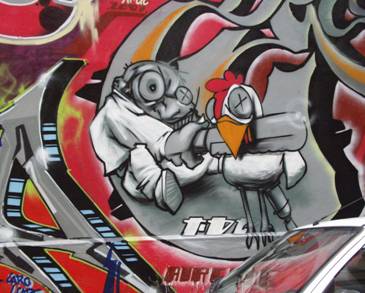
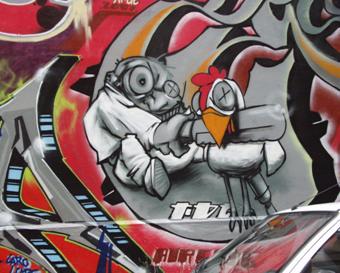
For the leuven benchmark, we observe that the key components are illumination and contrast. The first four matches again have relatively high accuracy, all AUC above 0.7. The sixth match has an AUC of zero, all false positives, and indicates that no features were matched correctly or no features were found in img6.ppm of leuven. This can be remedied by changing the threshold or incorporating contrast invariance.
bikes Benchmark
The bikes benchmark set includes images of the relatively same scene but at different resolutions. Our default for the designed descriptor is able to match well img1.ppm to img2.ppm, img3.ppm and img5.ppm. Our default descriptor is not invariant to changes in resolution.
wall Benchmark
The wall benchmark set presents images that are rotated and slightly scaled from one another. There is also a bit of skewing. However, there are many, distinct corners in this brick wall, making it amenable to corner searching. Because of this, our descriptor performed very well (invariance to rotation).
Strengths
From these tests, we know that
our default designed descriptor is rather invariant to rotation, as seen in the
wall benchmark set. The feature detection and matching algorithm works even better when distinct and unique corners are present. To a
degree, the descriptor is sufficient for differences in lighting and contrast,
but drops off quickly after a certain threshold (see leuven img1 and img6). Overall it seems to work well
with different illumination settings, but may need a change in thresholding or modifications to make it contrast
invariant. As shown from the
Weaknesses
The default designed descriptor does not account for extreme variations in contrast (leuven benchmark set), scaling (graf benchmark set), or resolution (bikes benchmark set). Moreover, only one out of the available three bands is used in this feature descriptor. Perhaps adding color information around the feature would increase greatly the positive matching rate.
Extra Credit Items
In addition to making a descriptor robust to changes in position, orientation and illumination, we incorporated methods to help the descriptor be robust to contrast, resolution, and scaling. We will address each in order.
We recognized from the leuven benchmark set that our method is not entirely robust to changes in contrast, namely between img1.ppm and img6.ppm with an AUC of 0. To that end, after subtracting the mean intensity from each descriptor, we also divided each pixel within the descriptor by the standard deviation. This in effect normalizes the distribution within descriptor, and thus makes it more robust to changes in contrast.
Contrast
Using this option in the designed descriptor, we computed an ROC curve and AUC
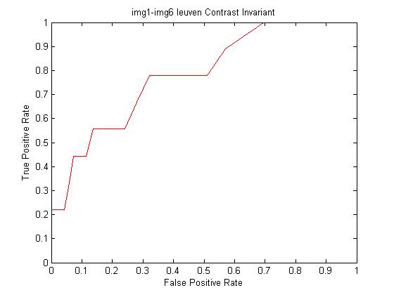
Calculated AUC: 0.780355
As we can see, by dividing by the standard deviation, the descriptor is much more robust to changes in contrast. The AUC increased from 0 to 0.780355 for matching leuven img1.ppm to img6.ppm.
Resolution
Moreover, we saw that the default designed descriptor that it was not very robust to changes in resolution (bikes img1.ppm, img4.ppm and img6.ppm). To remedy this, a 5x5 Gaussian mask was convolved with the original image three times. After each convolution, features were detected in the convolved image and recorded. In this way, hopefully changes in resolution would not effect the feature matching as much. First, we calculate the ROC curve and AUC for matching img1.ppm to img4.ppm, which before the modification had AUC of 0.581030. Doing so for img1.ppm and img4.ppm yields
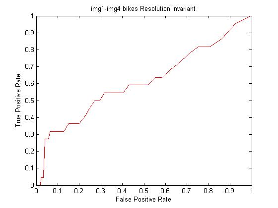
Calculated AUC: 0.607982
And again for img1.ppm to img6.ppm
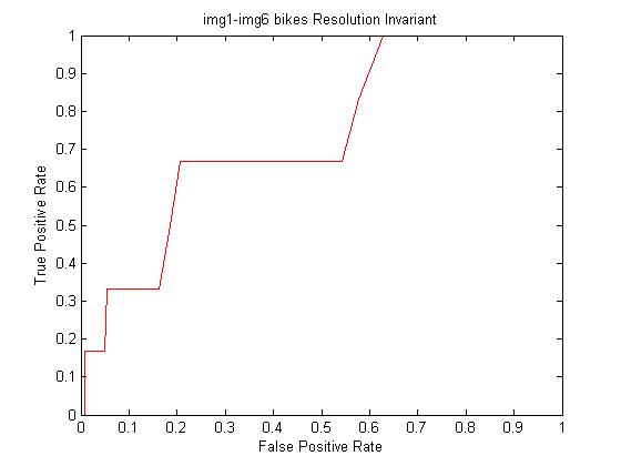
Calculated AUC: 0.734646
We see in both cases that by adding the Gaussian mask convolved images to the feature database increased the AUC, especially in the case of img1.ppm to img6.ppm.
Scale
Difference in scale could account for the poor AUC of 0.338889 in the graf benchmark set img1.ppm to img6.ppm. To account for scale, a pyramid of the original image was constructed. Namely, the image was made coarser and shrunk by a scale of 2 three separate times, resulting in images that were 2, 4 and 8 times smaller in edge length than the original image. Features were then detected in the smaller images and added to the feature database. Recalculating for graf img1.ppm to img6.ppm with the scale option, we obtain ROC graph and AUC
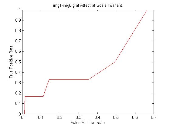
Calculated AUC: 0.285745
Unfortunately, this modification/option does not help with the graf benchmark set. In fact, the AUC decreased after applying this change. This could be due to a miscalculation in the scaling/pyramiding algorithm that I wrote, or because there is more than just scale involved when matching img1.ppm to img6.ppm.
Extra Images
In addition to the above given benchmark sets, we applied the developed feature detection and matching algorithm to a few other images. Three sets of other images are shown below
Fountain


In this set there is some rotation and scaling. Using the provided GUI, we detect features and attempt to match a few. It is somewhat successful

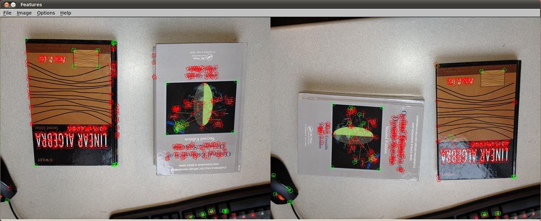
Books


With the books set, we should observe only translation and rotation. We anticipate that our algorithm will perform well, which it does, as shown below
Cat
and Apples

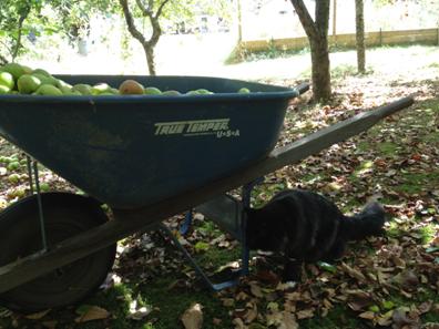
Finally, we take these images that are cluttered with many features and corners that are difficult to distinguish. We expect our algorithm won’t do so well, as shown below
