CSE576:
Project 1 Jeffrey
Herron Submitted
4/18/2013
1
Introduction:
This
project’s purpose is to demonstrate the effectiveness of different feature
detection, description, and matching methods. Two different descriptors were
implemented. The first was a simple five by five pixel window around any
detected corner. The second was a 15 by 15 window of pixels rotated to a
normalized axis with illumination-invariant pixel values. Furthermore, two
different matching methods were used to analyze the performance of these
descriptors. First we used standard Sum of Squared Distances (SSD) approach. A
second method was compared against SSD results that utilized a ratio metric.
Several images were used for performance measurement by means of examining the
Receiver Operator Characteristic (ROC) curve.
2
Feature Descriptors and Design Decisions:
As
mentioned above, the first feature descriptor consisted of a 5 pixel by 5 pixel
window around any point in the image where the Harris values exceeded a certain
threshold. This threshold was dynamically allocated to ensure a minimum number
of detected features while also ensuring a maximum amount of memory allocation.
The method consisted of the following steps:
1)
First convert
the image to a grayscale image.
2)
Compute the
Harris values for every point.
3)
Locate local
maxima within every 3 by 3 window above a certain threshold
4)
If there are too
many or too few features detected, update the threshold and repeat step #3. If
the threshold would become negative, proceed because all possible features have
been found.
5)
For every maxima
found in Step 3, save a 5 by 5 window centered on the pixel of interest.
From this simple schema, we can already tell that
this feature will not be very effective. This feature can truly only account
for simple translational changes and has very little rotational, scale, or
illumination invariance. To compute features in this way, the following command
should be executed in the directory containing the .exe:
Features computeFeatures
srcImage featurefile 3
The
second feature descriptor I implemented was significantly more complex and
accounts for rotational and illumination invariance, but does not account for
scalar changes. This primarily came down to problems implementing a pyramid
scheme as discussed in lecture notes. As before, the windows were centered on
points in an image where the Harris values exceeded a dynamic threshold.
However, unlike before, the pixel values in the window were divided by the
average pixel values to get a degree of illumination invariance. Furthermore,
the window was rotated such that all features would have the same primary
corner orientation. This would allow points of interest to be rotated in the
plane and still be successfully matched. Breaking this method into steps:
1)
Steps 1-4 are
the same as above.
5)
Filter the image
gradients to get less noisy gradient images.
6)
Calculate the
dominant corner orientation by using the atan2 function and the filtered x and
y gradient images.
7)
Take a 31 by 31
window around every point of interest
8)
Rotate the
window by the angle of the corner orientation
9)
Take the center
15 by 15 pixel window around the points of interest
10) Find the average pixel illumination
11) Divide every pixel by the average pixel illumination
In this way, we have a descriptor significantly more
robust to rotational and illumination variances. It should be noted, that since
I am only averaging the illumination across a window, I hope my features to be
more robust against localized illumination changes such shadows being cast by
potentially moving objects. To compute features in this way, the following
command should be executed in the directory containing the .exe:
Features computeFeatures
srcImage featurefile 2
3
Descriptor Performance:
To
test both of these descriptors, we first need to examine our Harris Values.
From there, we will examine the ROC with our primary interest being the area
under the curve (AUC) value. Furthermore, results from the benchmark tests will
also be presented.
3.1 Harris
Results
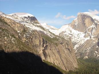
Firstly,
I would like to show two images and their corresponding Harris value images.
The first is a picture from Yosemite, then with the corresponding Harris
Values, and finally an image showing the localized threshold maximums:


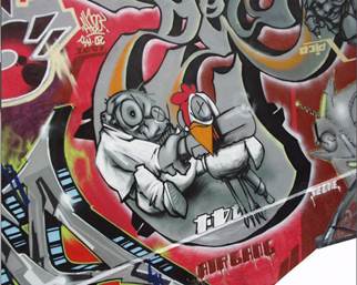
This
same analysis was done on a second set of images featuring some graffiti:

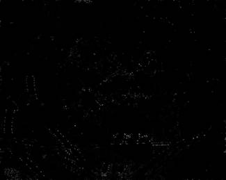

As
can be seen from the above images, we are successfully identifying points of
interest that correspond to corner areas. In the graffiti set particularly, the
corners of blue repeated structures are immediately obvious in the Harris
images.
3.2 ROC Test
Results
A
standard method of comparing the results of different descriptors and matching
algorithms is to examine the ROC curves. We examined the ROC curves for
matching two sets of image pairs with both descriptors outlined above. We
matched each of the feature files by using both SSD and Ratio matching.
Furthermore, we were provided with the SIFT ROC curves for the image sets. This
comes to a total of 6 ROC curves for each image pair to examine. Note that I
decided to use MATLAB to plot the ROC curves from the raw data primarily as a
cosmetic choice.
The Yosemite image pair have
only a translational relationship, so we should expect good performance from
each of the descriptors. Here are the two images:


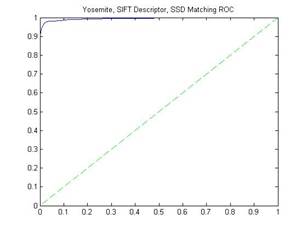
First, the ROC curves for the Yosemite pair with the
simple five pixels by five pixels feature descriptor using both SSD and Ratio
matching:


SSD AUC: 0.931849 Ratio AUC: 0.897590
Secondly, the ROC curves for the Yosemite pair with
the custom 15 pixel wide feature descriptor using both
SSD and Ratio matching:


SSD AUC: 0.956124 Ratio AUC: 0.972140
Finally, the ROC curves for the Yosemite pair with
the SIFT feature descriptor using both SSD and Ratio matching:

AUC values not given,
but are ~1
Next we will examine the ROC curves of the graffiti
images, which include a perspective rotational warp around the image due to a
change of viewpoint. This will be very hard for the 5 by 5 and my custom
descriptor to match. This is because there is no rotational invariance built
into the 5 by 5, and my custom descriptor is only invariant to planar
rotations. Here are the two images:

First, the ROC curves for the Yosemite pair with the
simple five pixels by five pixels feature descriptor using both SSD and Ratio
matching:


SSD AUC: 0.588724 Ratio AUC: 0.686437
Secondly, the ROC curves for the Yosemite pair with
the custom 15 pixel wide feature descriptor using both
SSD and Ratio matching:


SSD AUC: 0.769828 Ratio AUC: 0.863898
Finally, the ROC curves for the Yosemite pair with
the SIFT feature descriptor using both SSD and Ratio matching:


AUC values not given,
but are ~.95
In almost every case, the ratio matching
was better with the one exception was the Yosemite 5 by 5 descriptor. However,
the simple 5 by 5 descriptor’s weaknesses really show through when comparing it
against my custom descriptor and the SIFT descriptor. In every case it was
worse than either of the two. However, the custom descriptor cannot compare
against the performance shown by SIFT descriptor. In the graffiti images, the
weaknesses of not having any form or perspective invariance lead to
significantly worse results.
3.3 Benchmark
Results
To
test these two descriptors against even more images to understand their
weaknesses I utilized the benchmark feature of the Features.exe program. The
average AUC values for each image set are shown in the following table:
|
Image Set |
5by5, SSD
AUC |
5b5, Ratio
AUC |
Custom, SSD
AUC |
Custom,
Ratio AUC |
|
bikes |
0.34715 |
0.562370 |
0.459305 |
0.694549 |
|
graf |
0.39117 |
0.607535 |
0.687815 |
0.641050 |
|
leuven |
Error(=1.#IND00)? |
Error(=1.#IND00)? |
0.765866 |
0.861175 |
|
wall |
0.532012 |
0.634676 |
0.704273 |
0.831373 |
As
a quick aside, I have no idea why the five by five descriptor
has an error output. I’ve attempted to debug this with no avail. It would seem
that using the ROC command with these settings also returns this output.
Once again, we generally see that the
ratio performance is better than the SSD. Each of the images have
a varying set of differences between images we may want to match against. The
bike images progressively get blurrier, the graf
images have a perspective and rotational change, the leuven gets quite darker, and the wall has some shift
but also highly repeating structures. These results will be examined more
closely in the next section.
4
Additional Images and Performance:
To
further test my feature matching I took some additional images of items within
my home and then placed them within scenes. As a side note, since I know my
methods have no scale invariance I pre-scaled each of the item images to be
approximately the same size as the item within the scene. First I took a
picture of a DVD case and then placed it amongst other DVD cases. The two
originals are:


After pre-scaling the images so the DVD case would
be approximately the same size I then performed feature matching on it. First
using the simple descriptor:

Then I used my custom descriptor:

Qualitatively, the second image has a lot more
positive matches and less false positives. Note that both of these results are
shown within the features.exe GUI which does not allow threshold setting.
I also took some pictures of my cats in different
rooms and attempted feature recognition. Note that there are both
illumination, pose and rotational changes, however the size is
approximately the same so I did not pre-scale. The originals are:


First, the results of the simple descriptor
matching:

Second, the results of the custom descriptor
matching:
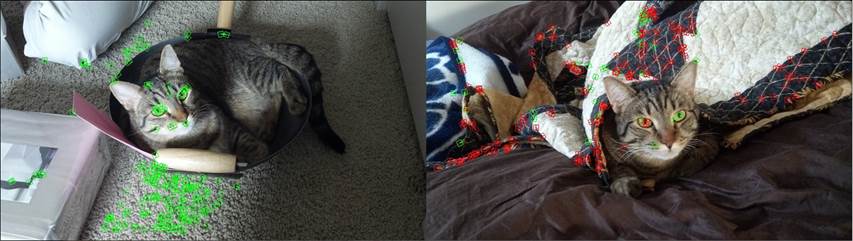
Qualitatively, both are pretty bad. Part of the
problem is that despite the stripes there are fewer features being found on the
cat’s face, so there are fewer features to match. While both have a pretty high
false positive to true positive rate, it seems as though there were more
correct matches made with the custom descriptor, but at this point it’s hard to
tell if that is a fluke or not.
5
Conclusions, Algorithm Strengths and Weaknesses:
The
performance test results can give us a glimpse into the strengths of the
different descriptors created in this project. The five-by-five window around
potential corners is fine for translations, however in the cases where there is
blurring, rotation, perspective shifts, contrast, or repeating structures, the
performance drops dramatically to in some cases below chance levels depending
on the matching method. While it has a small memory footprint and is easy to
program, it is just not useful for real world use.
The
custom descriptor I created for this project had significantly better
performance than the five-by-five descriptor. With some level of rotational and
illumination invariance as well as being significantly larger in dimensions
allowed it to be matched far more accurately. However, it still had problems
with the blurred images and the perspective shifts. This definitely gives me an
appreciation for the SIFT descriptor and how robust it is over such a wide
variety of variables that can exist between two images of the same item or
scene.
Furthermore,
it is interesting to see just how dramatic the results are after a change in
the matching function. The ratio matching was almost always better than the SSD
alone, except in the cases where both were doing pretty poorly anyway.
Overall
this was a very interesting project and it’s helpful to know what is actually
going on in the lower layers of the image recognition libraries. That being
said, I believe in the future I will stick to using more established feature
descriptor libraries such as SIFT rather than attempting to build my own.
Building a robust feature descriptor is hard, but in the case of this project
it was really fun and interesting.