CSE576 – Project 1
1
The DCT feature descriptor
1.1
Local Maxima
I use a partially adaptive local maxima threshold with pruning.
After computing all local maxima in a 3x3 window, I thin them out so that no local maximum is within 6 pixels of any other. This is done with a greedy algorithm that starts with the highest scoring local maximum and removes any others that are with the 6 pixel radius. Then, I select the next highest scoring that is left and repeat. Pruning in this manner ensures a more uniform spatial distribution of the features.
I choose to keep a minimum number of local maxima per image. The actual number selected is the maximum of the number above a hard-coded threshold number (empirically chosen), 2% of all local maxima, or 100 points. If there are less than 100 local maxima in the image, then all are chosen. This is done because a blurred image has features at the same location but with a lower Harris value. So by taking the top features instead of using a simple cut-off, loss of high frequency information has less of an impact on the resulting feature set.
1.2
DCT descriptor
My descriptor is quite simple. It contains the coefficients of a discrete cosine transform in a 25x25 window around a detected feature point. This results in a feature size of 625 elements. I discard the bias / DC offset coefficient and renormalize the remaining coefficients to have length 1.
My hope with testing the use of a DCT as a descriptor is that by converting an image region to frequency space we gain a few advantages. First, I believe that small misalignments will manifest as high frequency noise in the DCT and their effect will thus be minimized. Further, it is easy to cause the DCT to act as a low-pass filter by shrinking or eliminating the high frequency coefficients. However, I don't do this yet. Finally, removing the DC offset and normalizing intensity add robustness against changes in global illumination.
The DCT is straightforwardto implement and there is a good explanation at
this site.
2
Performance
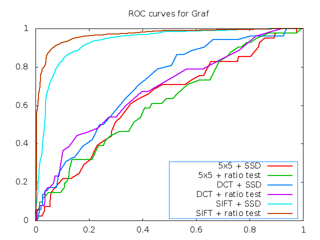
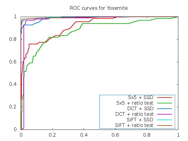
In general, the DCT descriptor outperforms the 5x5 descriptor quite well. For example, on the Yosemite test images, it approaches the performance of SIFT. However, it is not yet made rotationally invariant and that lack can be seen in its dismal performance on the graf benchmark set.
By discarding the DC coefficient and normlizing, the descriptor becomes nicely invariant to illumination changes, as can be seen in the results for leuven. It is also good for translational movement and slight amounts of rotation.
- Figure 1
-
Has 6 ROC curves for the graf test set.
- Figure 2
-
Has 6 ROC curves for the Yosemite test set.
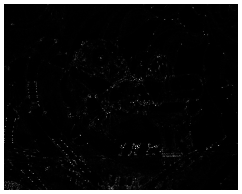
- Figure 3
-
Shows the output of the Harris operator for one of the images in the graf test set.
- Figure 4
-
Shows the output of the Harris operator for one of the images in the Yosemite test set.
- Table 1
-
Reports average AUC and error for SSD and Ratio tests for both 5x5 and DCT feature descriptors.
3
Future work
The DCT descriptor seems promising. I would like to test adding rotational invariance by calculating the center of mass of a feature and using it's offset from the center of the feature as a rotational normalizing component. Second, I'd like to see if the same results can be achieved using a reduced feature size by discarding some portion of the higher frequency coefficients. Finally, the DCT descriptor should be made scale invariant.
4
Figures
Table 1:
Benchmark, AUC scores for DCT features. * marks better score.