1. Feature Detector
The detector was implemented
according to the lecture notes.
Also, I computed their scale by applying 3
level pyramid of
Gaussian images.
Level 0: Original image
Level 1: Blurred and sub-sampled
image from the original image
Level 2: Blurred and sub-sampled
image from the lower level (level 2)
For each level, Harris operator was
applied and thus each pixel has 3 Harris values.
The maximum was selected as final Harris value for
each pixel and the level with the maximum value was assigned as the
scale of a feature point.
2. Feature Descriptor
I tried 3 different descriptors
(1) Simple 5X5 windows
It simply
samples 25 pixels from 5X5 window centered on detected interesting
points.
(2) MOPS
I have
implemented MOPS feature descriptor as explained in [1] and lecture
notes.
(1) Compute the angle of a feature point using X- and Y-axis
gradients.
(2) Put
40X40 window on a feature point.
(3) Align the
window horizontally, i.e, rotate the patch according to the angle.
(4) Subsample
9X9 pixels from the 40X40 patches. Originally, they used 8X8
sub-sampled pixels.
If the interesting point is detected at pyramid
level l, pixels are
sub-sampled from (l+1) level
pyramid
image.
(5) Normalize
the descriptor by subtracting the mean from its elements and dividing
them
by the standard deviation.
(3) Simple Histogram of Gradient
I have
implemented a simple version of Histogram of Gradient (SHoG).
(1) Compute X- and Y-axis
gradients for an input image.
(2) Put 10X10
window on a feature point.
(3) Construct
18-bin orientation histogram by accumulating the magnitudes
according to angles of feature points.
If the interesting point is detected at pyramid
level l, magnitudes are
obtained from l-level
pyramid
image.
(4) Circularly
shift the bins so that a bin with the maximum magnitude becomes a first
bin in a histogram.
(5) Normalize
the histogram by its maximum value.
3. Design and Implementation Issue
(1) For the feature detector, I used pyramid of Gaussian images.
At first, I applied the feature detection procedure
without pyramid of Gaussian images,
but it could barely detect interesting
points from bike image 5 and 6 because they are too much blurred.
After thresholding the images, almost no feature points were obtained
from the
image of zero level (the left-most image).
After applying Pyramid of Gaussian images, I could obtain some feature
points.
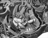
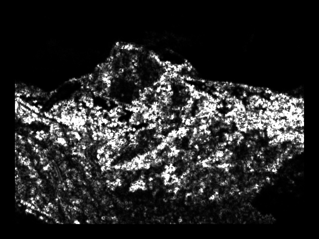
The following images show pyramid of images and their Harris
values. They are multiplied by 1,000 to make them more visible.


Level 0
Level 1
Level 2
< Pyramid of Gaussian Images: Bikes
6>


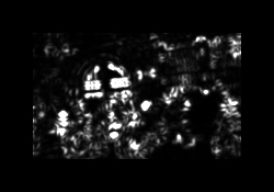
Level 0
Level 1
Level 2
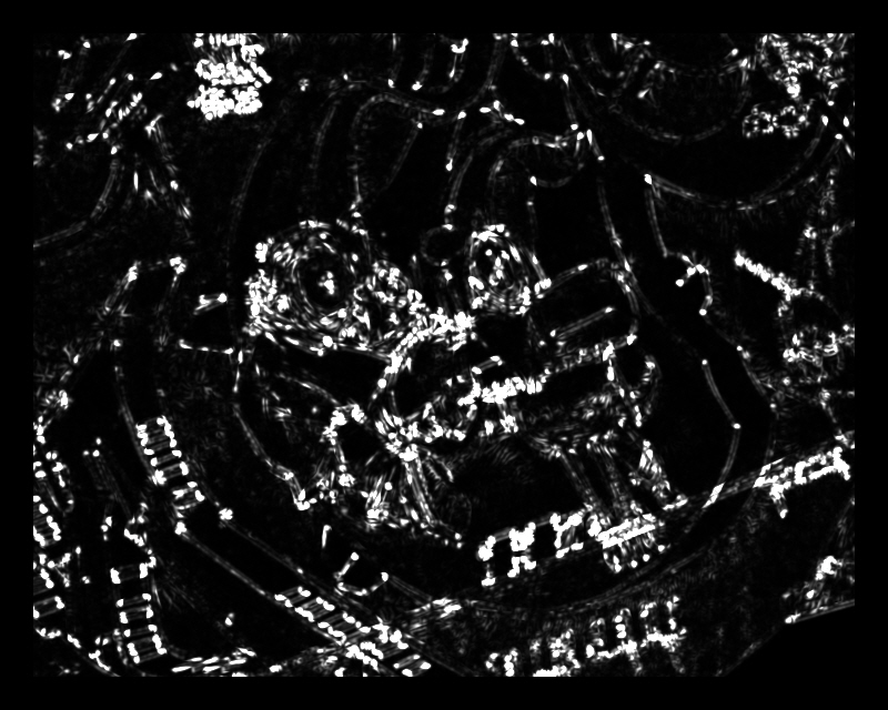
<
Harris Images: Bikes 6>
(2) To calculate gradients, I used first derivative of Gaussian instead
of the Sobel operator.
It is well known that the derivative of Gaussian is more robust to
noise than the Sobel operator.
In real implementation, 5X5 window was employed.

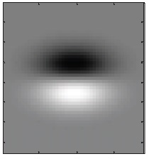
<First
Derivative of Gaussian Filter>
(3) The given skeleton codes had some bugs in 'Convolve()' function.
It probably did not affect the algorithm's performance too much,
but the original codes did not work at all with 'UpLevel()'
function in Pyramid class.
I had modified the codes using my own found bugs and with help
from the posting of Jefferey.
Modified Codes:
double sum = 0;
for (int k = 0; k < kShape.height; k++)
{
for (int l = 0; l <
kShape.width; l++)
{
/* Original
Codes
if ((x-kernel.origin[0]+k >= 0) && (x-kernel.origin[0]+k < sShape.width) &&
(y-kernel.origin[1]+l >= 0) && (y-kernel.origin[1]+l < sShape.height))
{
sum += kernel.Pixel(k,l,0) * src.Pixel(x-kernel.origin[0]+k,y-kernel.origin[1]+l,c);
}
*/
// Modified
Codes
if ((x+kernel.origin[0]+l >= 0) && (x+kernel.origin[0]+l < sShape.width) &&
(y+kernel.origin[1]+k >= 0) && (y+kernel.origin[1]+k < sShape.height))
{
sum += kernel.Pixel(l,k,0) * src.Pixel(x+kernel.origin[0]+l,y+kernel.origin[1]+k,c);
}
}
}
dst.Pixel(x,y,c) = (T) __max(dst.MinVal(),
__min(dst.MaxVal(), sum));
4. Performance Report for Graf and Yosemite
(1) Harris Images for Graf and Yosemite
The following images show pyramid of images and their Harris
values. They are multiplied by 1,000 to make them more visible.
Harris scores was multiplied by 1,000 to make it more visible.


Level 0
Level 1
Level 2
Level 0
Level 1
Level 2


Level 0
Level 1
Level 2
Level 0
Level 1
Level 2
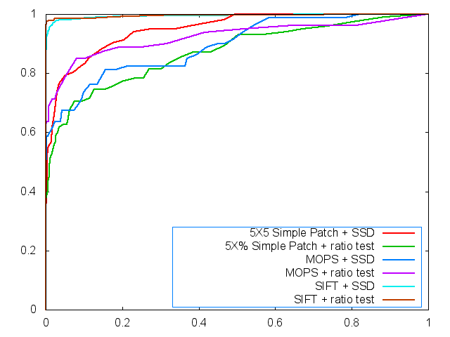
(2) AUC and ROC for Graf and Yosemite with MPOS Descriptor
There are the test results using the MPOS descriptor.
|
Simple 5X5 Window |
MPOS |
|
SSD |
Ratio |
SSD |
Ratio |
| Graf |
0.601380 |
0.716935 |
0.767863 |
0.840617 |
| Yosemite |
0.949337 |
0.871425 |
0.893986 |
0.922928 |
< AUC with MPOS Feature
Descriptor>

<Graf>
<Yosemite>
< ROC with
MPOS Descriptor>
(3) AUC and ROC for Graf and Yosemite with SHoG Descriptor
There are the test results using the SHoG descriptor.
|
Simple 5X5 Window |
SHoG |
|
SSD |
Ratio |
SSD |
Ratio |
| Graf |
0.601380 |
0.716935 |
0.707428 |
0.505639 |
| Yosemite |
0.949337 |
0.871425 |
0.806369 |
0.776603 |
< AUC with MPOS Feature
Descriptor>


< ROC with
SHoG Descriptor>
5. Performance Report for Benchmark Datasets using
MOPS Descriptor
(1) AUC for MOPS
|
Bikes |
Graf |
Leuven |
Wall |
|
Simple 5X5 |
MOPS |
Simple 5X5 |
MOPS |
Simple 5X5 |
MOPS |
Simple 5X5 |
MOPS |
|
SSD |
Ratio |
SSD |
Ratio |
SSD |
Ratio |
SSD |
Ratio |
SSD |
Ratio |
SSD |
Ratio |
SSD |
Ratio |
SSD |
Ratio |
| 1 to 2 |
0.520477 |
0.646873 |
0.836848 |
0.878549 |
0.601380 |
0.716935 |
0.767863 |
0.840617 |
0.400132 |
0.615837 |
0.856909 |
0.899898 |
0.588455 |
0.698919 |
0.913984 |
0.919485 |
| 1 to 3 |
0.537866 |
0.682949 |
0.858690 |
0.845195 |
0.533435 |
0.691536 |
0.785318 |
0.823008 |
0.197313 |
0.634088 |
0.869978 |
0.850670 |
0.561754 |
0.685365 |
0.906628 |
0.899969 |
| 1 to 4 |
0.630400 |
0.721574 |
0.916821 |
0.920720 |
0.564011 |
0.647527 |
0.631655 |
0.721040 |
0.352941 |
0.693137 |
0.885851 |
0.934788 |
0.543599 |
0.616714 |
0.875732 |
0.884777 |
| 1 to 5 |
0.567745 |
0.573099 |
0.881388 |
0.829583 |
0.448628 |
0.594624 |
0.552447 |
0.672306 |
0.045010 |
0.678082 |
0.934653 |
0.950786 |
0.415668 |
0.612473 |
0.796353 |
0.817903 |
| 1 to 6 |
0.469473 |
0.489226 |
0.928649 |
0.872378 |
0.631706 |
0.468822 |
0.745902 |
0.525956 |
0.037182 |
0.580235 |
0.858076 |
0.888039 |
0.442719 |
0.469540 |
0.769981 |
0.651870 |
| Average |
0.545192 |
0.622744 |
0.884479 |
0.869285 |
0.555832 |
0.623889 |
0.696637 |
0.716585 |
0.206516 |
0.640276 |
0.881093 |
0.904836 |
0.510439 |
0.616602 |
0.852536 |
0.834801 |
(2) Average Pixel Error for MOPS
|
Bikes |
Graf |
Leuven |
Wall |
|
Simple 5X5 |
MOPS |
Simple 5X5 |
MOPS |
Simple 5X5 |
MOPS |
Simple 5X5 |
MOPS |
|
SSD |
Ratio |
SSD |
Ratio |
SSD |
Ratio |
SSD |
Ratio |
SSD |
Ratio |
SSD |
Ratio |
SSD |
Ratio |
SSD |
Ratio |
| 1 to 2 |
252.216521 |
* |
192.850547 |
* |
216.762120 |
* |
214.352871 |
* |
320.073363 |
* |
208.402465 |
* |
287.496260 |
* |
245.638696 |
* |
| 1 to 3 |
287.574315 |
* |
218.918309 |
* |
215.334316 |
* |
216.680018 |
* |
348.562424 |
* |
238.799857 |
* |
302.244337 |
* |
269.444685 |
* |
| 1 to 4 |
291.947181 |
* |
251.195576 |
* |
249.902211 |
* |
258.476088 |
* |
364.481320 |
* |
272.263070 |
* |
326.551455 |
* |
321.830911 |
* |
| 1 to 5 |
316.373814 |
* |
271.870703 |
* |
231.255573 |
* |
279.467612 |
* |
357.773007 |
* |
278.659521 |
* |
397.561260 |
* |
348.350584 |
* |
| 1 to 6 |
323.488355 |
* |
292.244289 |
* |
250.132000 |
* |
293.201983 |
* |
387.338809 |
* |
304.072435 |
* |
384.408618 |
* |
386.268992 |
* |
| Average |
294.320037 |
* |
245.415885 |
* |
232.677244 |
* |
252.435714 |
* |
355.645785 |
* |
260.439469 |
* |
339.652386 |
* |
314.306774 |
* |
Note: * indicates that a value is equal to that of its left cell.
6. Performance Report for Benchmark Datasets using SHoG Descriptor
(1) AUC for SHoG
|
Bikes |
Graf |
Leuven |
Wall |
|
Simple 5X5 |
SHoG |
Simple 5X5 |
SHoG |
Simple 5X5 |
SHoG |
Simple 5X5 |
SHoG |
|
SSD |
Ratio |
SSD |
Ratio |
SSD |
Ratio |
SSD |
Ratio |
SSD |
Ratio |
SSD |
Ratio |
SSD |
Ratio |
SSD |
Ratio |
| 1 to 2 |
0.520477 |
0.646873 |
0.759675 |
0.779799 |
0.601380 |
0.716935 |
0.707428 |
0.505639 |
0.400132 |
0.615837 |
0.812513 |
0.834165 |
0.588455 |
0.698919 |
0.640223 |
0.721789 |
| 1 to 3 |
0.537866 |
0.682949 |
0.780198 |
0.824691 |
0.533435 |
0.691536 |
0.608422 |
0.465565 |
0.197313 |
0.634088 |
0.783544 |
0.811488 |
0.561754 |
0.685365 |
0.612144 |
0.690030 |
| 1 to 4 |
0.630400 |
0.721574 |
0.796617 |
0.838308 |
0.564011 |
0.647527 |
0.586530 |
0.504566 |
0.352941 |
0.693137 |
0.781254 |
0.726508 |
0.543599 |
0.616714 |
0.503173 |
0.562073 |
| 1 to 5 |
0.567745 |
0.573099 |
0.833663 |
0.729997 |
0.448628 |
0.594624 |
0.799040 |
0.740055 |
0.045010 |
0.678082 |
0.736864 |
0.761121 |
0.415668 |
0.612473 |
0.425575 |
0.452103 |
| 1 to 6 |
0.469473 |
0.489226 |
0.885151 |
0.790604 |
0.631706 |
0.468822 |
0.159153 |
0.304645 |
0.037182 |
0.580235 |
0.712928 |
0.718311 |
0.442719 |
0.469540 |
0.548355 |
0.713902 |
| Average |
0.545192 |
0.622744 |
0.811061 |
0.792680 |
0.555832 |
0.623889 |
0.572115 |
0.504094 |
0.206516 |
0.640276 |
0.765421 |
0.770319 |
0.510439 |
0.616602 |
0.545894 |
0.627979 |
(2) Average Pixel Error for SHoG
|
Bikes |
Graf |
Leuven |
Wall |
|
Simple 5X5 |
SHoG |
Simple 5X5 |
SHoG |
Simple 5X5 |
SHoG |
Simple 5X5 |
SHoG |
|
SSD |
Ratio |
SSD |
Ratio |
SSD |
Ratio |
SSD |
Ratio |
SSD |
Ratio |
SSD |
Ratio |
SSD |
Ratio |
SSD |
Ratio |
| 1 to 2 |
252.216521 |
* |
224.492398 |
* |
216.762120 |
* |
258.299126 |
* |
320.073363 |
* |
229.540048 |
* |
287.496260 |
* |
294.649230 |
* |
| 1 to 3 |
287.574315 |
* |
232.872365 |
* |
215.334316 |
* |
249.911122 |
* |
348.562424 |
* |
272.130749 |
* |
302.244337 |
* |
301.220350 |
* |
| 1 to 4 |
291.947181 |
* |
262.912727 |
* |
249.902211 |
* |
285.863968 |
* |
364.481320 |
* |
303.092765 |
* |
326.551455 |
* |
321.936495 |
* |
| 1 to 5 |
316.373814 |
* |
277.228958 |
* |
231.255573 |
* |
290.280118 |
* |
357.773007 |
* |
336.119879 |
* |
397.561260 |
* |
353.715023 |
* |
| 1 to 6 |
323.488355 |
* |
295.312835 |
* |
250.132000 |
* |
290.160905 |
* |
387.338809 |
* |
344.569287 |
* |
384.408618 |
* |
383.460122 |
* |
| Average |
294.320037 |
* |
258.563857 |
* |
232.677244 |
* |
274.903048 |
* |
355.645785 |
* |
297.090545 |
* |
339.652386 |
* |
330.996244 |
* |
Note: * indicates that a value is equal to that of its left cell.
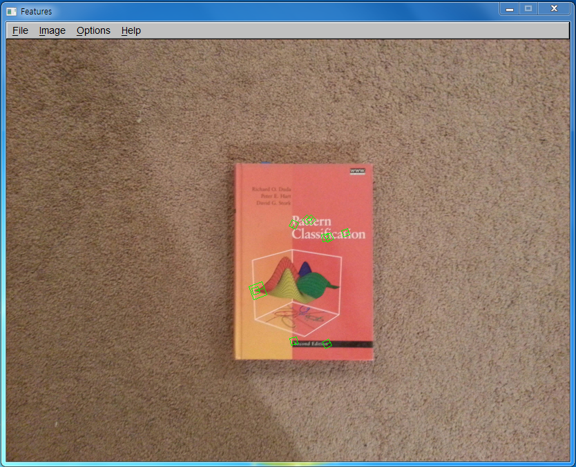
7. My Own Pictures
I took 4 pictures and performed object search experiment.
In the following pictures, the image in the first row is a query image
and a database has 3 images.
The image in the last row shows the search results with a query.

<Query>


<Images in Database>
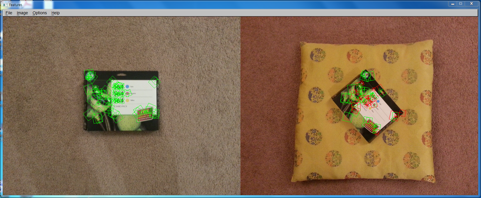
<Search result>
8. Strengths and Weaknesses
(1) The feature detector is scale-invariant since pyramid of
Gaussian images was applied. Please, refer to Section 3.(1).
(2) Instead of the Sobel operator, the derivative of Gaussian was used
to calculate image gradients, which is more robust to noise.
Note that image gradients are used in many parts in this project. It is
used to calculate Harris values, the orientation of feature points and
feature descriptors.
Please, refer to Section 3.(2).
(3) The MOPS descriptor is robust to changes:
in scale because pyramid of Gaussian images
was applied. It can be confirmed by the test results for Bikes datasets
in Section 5.(1)
in position because the information contained
in a pixel (gray value) is spread to its neighbors by blurring pixels
using Gaussian filter.
in orientation because the 40X40 window is
aligned horizontally according to the angle of a feature point.
in illumination (or contrast)
because subsampled pixels are normalized by their mean and
standard deviation. It can be confirmed by the test results for Leuven
datasets in Section 5.(1).
(4) The SHoG descriptor is robust to changes:
in scale because pyramid of Gaussian images
was applied. It can
be confirmed by the test results for Bikes datasets in Section 5.(2)
in position because the descriptor is based
on histogram. However, it loses spatial information.
in orientation because the feature descriptor
is aligned so that a bin with the maximum magnitude becomes a
first bin in a histogram.
in illumination (or contrast) because the
descriptor is based on image gradients, which are calculated by
relative difference between pixels. It can
be confirmed by the test results for Leuven datasets in Section 5.(2)
9. Extra Credit
Please refer to the explanation in Section 8.
(1) The implemented features are contrast invariant.
(2) The feature detector is scale invariant.
(3) Two additional feature descriptors were implemented and compared
with the simple 5X5 window descriptor.
10. Command Argument
| Feature Type |
Option Value |
| Simple 5X5 Window |
2 |
| MOPS |
3 |
| SHoG |
7 |
| Match Type |
Option Value |
| SSD |
1 |
| Ratio Test |
2 |
Reference
[1] Multi-Image Matching using Multi-Scale Oriented Patches