Computer Vision (CSEP 576), Winter 2005

Project 4: Eigenfaces

Uri Finkel

Testing recognition with cropped class images

The average face and the first 10 eigenfaces x400%:

Average Face:

Eigenface#1	Eigenface#2	Eigenface#3	Eigenface#4	Eigenface#5


Eigenface#6	Eigenface#7	Eigenface#8	Eigenface#9	Eigenface#10

2. Plot of the number of faces correctly recognized versus the number of eigenfaces used:

Looking at graph no. 1, we see that the first few eigenfaces make a great difference on the recognition solutions, but after that the addition of each eigenface has little or no impact on how many faces are recognized. This follows is due to the fact that the most important eigenfaces (with the largest eigenvalue) are at the head of the list. The later eigenfaces keep track of more minor facial features and do not contribute significantly to the reconstructed face. The disadvantage of using a large number of eigenfaces is the performance and the storage size of the user database.

The trend of data points in graph no. 1 shows an asymptotic curve; its slope rises sharply at the beginning, but then tapers off, and eventually approaches 0. A good way to find the optimal number of eigenfaces is to find the point that divides the steep slope of the curve from the shallow slope. A mathematical way to find this point is to find the point along the curve at which the derivative is 1, that is, the part of the curve whose tangent is a 45-degree angle. The number of eigenfaces at this point would be a good number of eigenfaces to use. In this particular instance, about 5 eigenfaces looks like a good candidate.

Even with 31 eigenfaces, only about 67% of the faces in the dataset were successfully recognized. Here is an example of two faces that were not successfully recognized even with 31 eigenfaces (images are normalized and at 300% zoom):

Original smiling face	Projection of the Original face	Misrecognized as	Should have been (non smiling face)

The projections seem somewhat reasonable-looking as a non-smiling version of the original face, but what's interesting is that in the first case someone without mustache is recognized as someone with mustache, and in the second case someone without glasses is recognized as someone with glasses. However, you can see that the misrecognized faces seem to have roughly the same orientation and head tilt angle within the window, and this probably contributed a lot to the match. The correct match for the first face appeared at the 3^rd position, and the correct match for the second face was at position #10.

Cropping and finding faces

1. Crop of bush_george_w_portrait.tga image using min_scale,max_scale, step parameters of .25, .55, .01.

bush_george_w_portrait.tga	Croped results x2

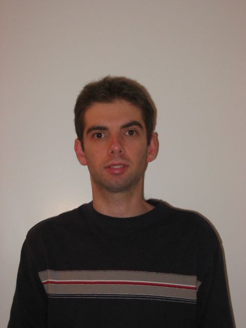
2. Crop of a digital picture of myself using min_scale,max_scale, step parameters of .15, .30, .01.

Uri_Finkel.tga	Cropped results

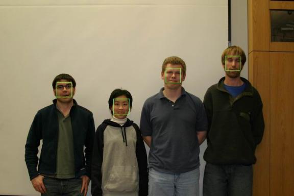
3. Find faces in IMG_8270.tga using the mark (crop=false) option, n=4, min_scale=0.62, max_scale=0.64 and step=0.02.

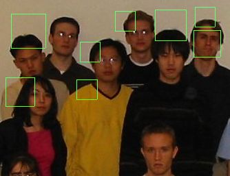
4. As a second picture I used half of the group picture of last year’s course.

I did some experiments to try and get the best results.

First I tried it with my original Code and MSE calculation (the standard) using the mark (crop=false) option, n=8, min_scale=0. 5, max_scale=0.8 and step=0.05.

Then I decided to try it on the same scale with the modified MSE calculation (“One possible approach is to multiply the MSE by the distance of the face from the face mean and then dividing by the variance of the face.”).

As you can see it did not improved the solution.

Then I decided to go back to the first solution and to try to prevent the algorithm from getting fooled by low-texture areas, by blurring the picture with Gaussian filter, but it did not improve the results.

Then I decided to take the color thresholds approach, and to try and minimize the mismatches by processing only pixels with skin color. In order to decide the initial values and thresholds for each channel (RGB) I sampled a few pictures.

The best match turned out, using the original MSE with no additional improvements.

There are several reasons why 2 of the 8 faces failed to be identified:

1. Some of the faces are slightly tilted at an angle (the back row). Since each window is projected into face-space without rotation, and since none of the eigenfaces exhibit much tiltedness, this would cause misalignments of features.

2. Each window in the image measured 25x25 pixels, since the eigenfaces were 25x25. In creating the eigenfaces, all the test images were distorted to fit into this square window. However, the faces from the image are taken as is. This is going to cause error on anyone whose facial features do not align to the square distortion exhibited within the eigenfaces. For example, the person's face on the right front side of the first row probably doesn’t match well with these scrunched square faces.

3. The training dataset needs to consist of many, many more faces with wide diversity, in order to yield better results.

Why do the miscalculated windows lie where they do? Well, the error associated with each window is equal to its MSE. I have noticed from the debug face map that the following areas seem to “look” like faces in the faces plane.

1. The area between the shirt and the neck.

2. Lightly textured backgrounds or surfaces with little intensity difference. Once normalized, these segments tend to turn into gradients that are approximated surprisingly well by the eigenfaces.

3. Other areas of clothing, which for whatever reason or another, show up as a face.

From looking at MSE values, the problem seems to be less that these areas make good faces, but that the real faces aren't making good faces. This is a problem that could possibly be rectified by a larger training set.

As far as choosing the scale ranges over which to search each group image, I found that a good technique was to open the image in Irfanview, draw boxes around a couple of the faces, and divide the width and height of these boxes by the width and height of the search windows (25x25).

Extra Credit:

I implemented the verifyFace method and here are my findings:

MSE	Correct Match	False negative	False positive	Total False
5000	4	27	0	27
15000	8	23	0	23
25000	12	19	1	20
50000	15	16	1	17
75000	23	8	6	14
100000	24	7	9	16

The best-performing MSEs are the ones with the minimum total number of falses. This means that MSEs of 75000 give the best performance, with total of 14 false error rate of 45%.